HFW 10: When average wins

An average growth rate forecast model beats the more sophisticated models thus far

In our last Hello Forecasting World post, we introduced growth rate forecasting as a prelude to discussing models designed to handle heteroskedasticity, a common problem in time-series forecasting. What is heteroskedasticity? It’s a phenomenon where the error terms in the forecast are not constant. Super helpful right? The key concept here is, when forecasting you want the errors to be random and stationary; plotted, they essentially look like a wide, spread out cloud that has a pretty constant height. If, instead, the error terms look like a tornado or shotgun shot, then you've got a problem. Without going too deep into the statistics, if you've got this hetero whatever, then your estimates are likely to be biased or unreliable. Suffice it to say, you shouldn’t put much confidence in the confidence and prediction intervals. Now if you don't really care about the statistics and just want to hack your forecast, you can calculate the error rate and figure out some way to push the errors closer to zero using brute force iteration. However, with univariate time series, such as we're working with here, that won't get you results much different than a linear regression. So we need a different hack. Let's get to the data!

The last post used the most recent sequential change in revenues in our S&P 500 sector dataset to forecast the next four quarters of revenues. Essentially, we're performing recursive forecasting again, where the output of the last value is used as the input for the next forecast. We showed the scaled root mean-squared error graph in the last post. We then promised to compare the results with our benchmark models. Here's that output.

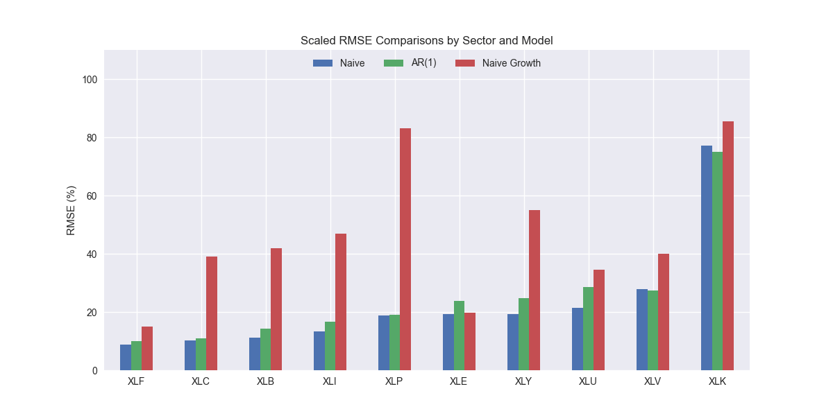
That looks pretty atrocious. We can, of course, understand why. There's no seasonality baked in and even equity research analysts know that revenues don't compound in a straightline fashion for most companies. We all wish they did so we could buy those stocks. But that's not how things happen.

It's interesting that the truly naïve model continues to perform well even against a slightly more sophisticated naïve model—the forecasting version of jumbo shrimp. A slightly less naïve model might use the last four year-over-year growth rates instead of the last sequential growth rate to forecast revenues. That would look like the following.

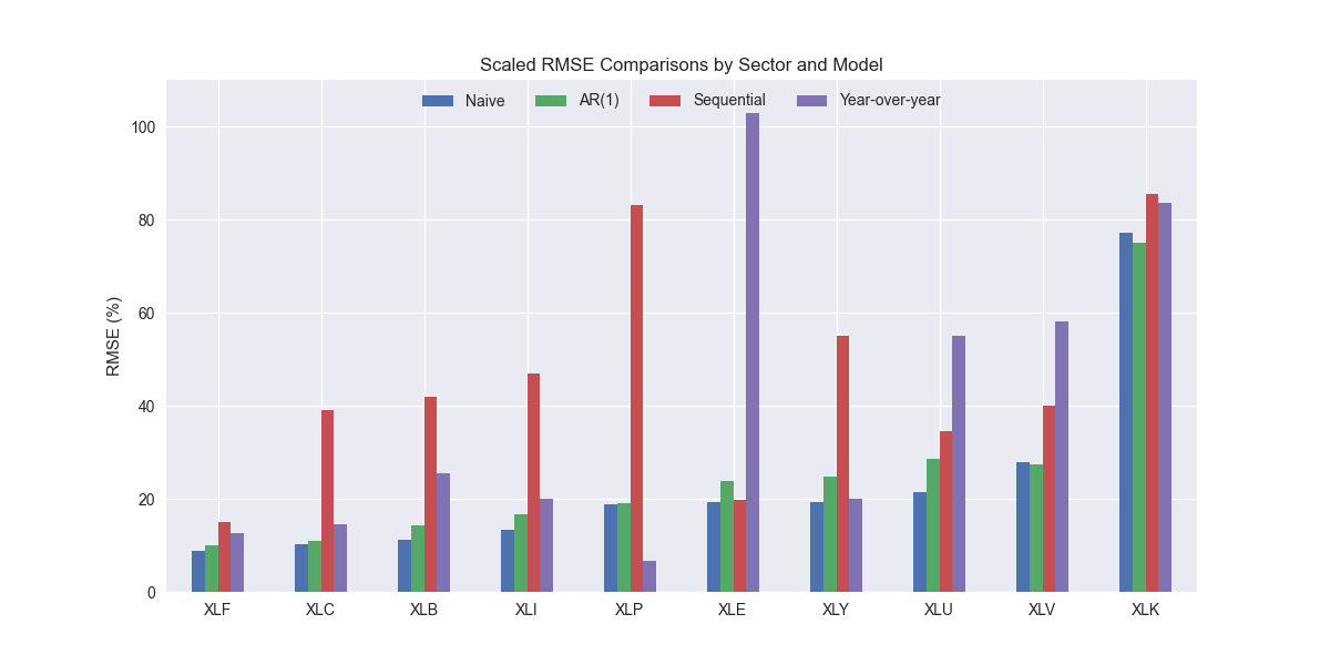
This method does show some improvement vs. the naïve growth rate forecast. But it is still worse than the truly naïve and the AR(1) models. Even removing the XLE outlier we still get an error rate above the benchmarks.

Let's add one more model to the mix. For this semi-naïve model, we'll take the average growth rate over the training period and apply that recursively to our forecasts. Plot below.

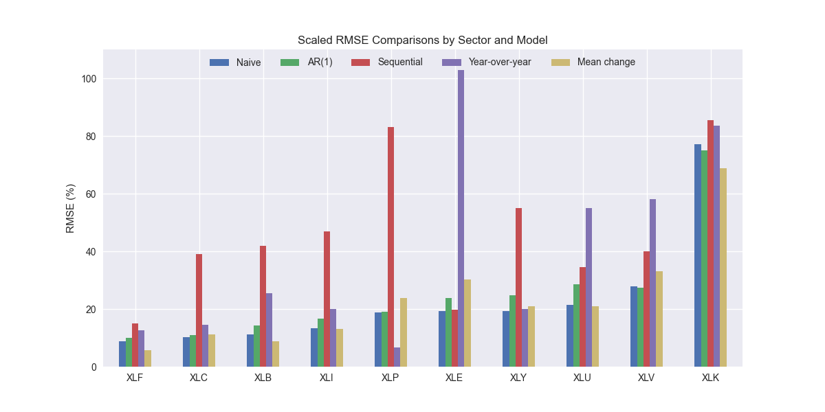
Interestingly, this model performs much better than the other naïve growth rate models and relatively well compared to the benchmark models. Indeed, it's average error rate across all the sectors is below the AR(1) model and only 1% point worse than the naïve.

What are the takeaways? Again, note how some models perform better on specific sectors even if in aggregate they are worse than the benchmarks. Applying a simple average growth rate to forecast revenues, yields the best model, beating out all of the sophisticated models we’ve discussed so far and only fractionally missing the naïve model's performance. Critically, if we were to graph the average growth rate forecasts, we'd expect them to look a lot better than the naïve model. This is important because if you were presenting a forecast to stakeholders, you'd probably get a very poor reception if you recommended a naïve forecast, even if it were the best performing model. Now that we've introduced the basics of using growth rates to forecast revenues, we can use some of the previous models like AR and ARMA on growth rates, which will then set us up nicely to tackle heteroskedasticity! Don't hold your breath! Stay tuned!

Code below

# Load packages
import pandas as pd
import numpy as np
from datetime import datetime, timedelta
import statsmodels.api as sm
import matplotlib.pyplot as plt
from matplotlib.ticker import FuncFormatter
import matplotlib as mpl
import pickle

# Assign chart style
plt.style.use('seaborn-v0_8')
plt.rcParams["figure.figsize"] = (12,6)

# Handy functions 
def save_dict_to_file(data, filename):
    with open(filename, 'wb') as f:
        pickle.dump(data, f)

def load_dict_from_file(filename):
    with open(filename, 'rb') as f:
        return pickle.load(f)

def get_rmse_dataframe(model_dict, rev_dict, start, end, dynamic=True):
    err_df = pd.DataFrame(columns = ['sector', 'ticker', 'actual', 'predicted'])
    count = 0
    for key in model_dict:
        for ticker in model_dict[key]:            
            try: 
                y_act = rev_dict[key][ticker].values
                if dynamic:
                    y_pred = model_dict[key][ticker].predict(start,end, dynamic=False).values
                else:
                    y_pred = model_dict[key][ticker].predict(start,end).values
            except ValueError as e:
                print(f"{ticker} fails due to {e}")
                y_act = np.nan
                y_pred = np.nan

            err_df.loc[count] = [key.upper(), ticker, y_act, y_pred]
            count += 1

    for ticker in err_df['ticker'].to_list():
        actual = err_df.loc[err_df['ticker']==ticker, 'actual'].values[0]
        predicted = err_df.loc[err_df['ticker']==ticker, 'predicted'].values[0]
        rmse = np.sqrt(np.mean((actual - predicted)**2))
        rmse_scaled = rmse/actual.mean()
        err_df.loc[err_df['ticker']==ticker, 'rmse'] = rmse
        err_df.loc[err_df['ticker']==ticker, 'rmse_scaled'] = rmse_scaled

    return err_df

def get_rmse_scaled(series):
    return np.sqrt(np.mean((series['actual']-series['predicted'])**2))/np.mean(series['actual'])

def flatten_df(dataf: pd.DataFrame, group_name:str, cols:list) -> pd.DataFrame:
    df_grouped = dataf.groupby(group_name)[cols].agg(list)

    for col in cols:
        df_grouped[col] = df_grouped[col].apply(lambda x: np.concatenate(x))
    
    df_long = df_grouped.apply(pd.Series.explode).reset_index()

    return df_long

# Symbols used
etf_symbols = ['XLF', 'XLI', 'XLE', 'XLK', 'XLV', 'XLY', 'XLP', 'XLB', 'XLU', 'XLC']

ticker_list = ["SHW", "LIN", "ECL", "FCX", "VMC",
               "XOM", "CVX", "COP", "WMB", "SLB",
               "JPM", "V", "MA", "BAC", "GS",
               "CAT", "RTX", "DE", "UNP", "BA",
               "AAPL", "MSFT", "NVDA", "ORCL", "CRM",
               "COST", "WMT", "PG", "KO", "PEP",
               "NEE", "D", "DUK", "VST", "SRE",
               "LLY", "UNH", "JNJ", "PFE", "MRK",
               "AMZN", "SBUX", "HD", "BKNG", "MCD",
               "META", "GOOG", "NFLX", "T", "DIS"
]

xlb = ["SHW", "LIN", "ECL", "FCX", "VMC"]
xle = ["XOM", "CVX", "COP", "WMB", "SLB"]
xlf = ["JPM", "V", "MA", "BAC", "GS"]
xli = ["CAT", "RTX", "DE", "UNP", "BA"]
xlk = ["AAPL", "MSFT", "NVDA", "ORCL", "CRM"]
xlp = ["COST", "WMT", "PG", "KO", "PEP"]
xlu = ["NEE", "D", "DUK", "VST", "SRE"]
xlv = ["LLY", "UNH", "JNJ", "PFE", "MRK"]
xly = ["AMZN", "SBUX", "HD", "BKNG", "MCD"]
xlc = ["META", "GOOG", "NFLX", "T", "DIS"]

sectors = [xlf,  xli,  xle,  xlk, xlv,  xly, xlp, xlb, xlu, xlc]

# Sector dictionary
sector_dict = {symbol.lower(): tickers for symbol, tickers in zip(etf_symbols, sectors)}

# Load data from disk
# See Code Walk-Throughs for how we built the data set
df_sector_dict = load_dict_from_file("hello_world/data/simfin_df_rev_dict.pkl")

# Create functions for indexing
def create_index(series):
    if series.iloc[0] > 0:
        return series/series.iloc[0] * 100
    else:
        return (series - series.iloc[0])/-series.iloc[0] * 100

# Clean dataframes
df_rev_index_dict = {}
for key in sector_dict:
    temp_df = df_sector_dict[key].copy()
    col_1 = temp_df.columns[0]
    temp_df = temp_df[[col_1] + [x for x in temp_df.columns if 'revenue' in x]]
    temp_df.columns = ['date'] + [x.replace('revenue_', '').lower() for x in temp_df.columns[1:]]
    temp_idx = temp_df.copy()
    temp_idx[[x for x in temp_idx if 'date' not in x]] = temp_idx[[x for x in temp_idx if 'date' not in x]].apply(create_index)
    df_rev_index_dict[key] = temp_idx

# Create train/test dataframes
df_rev_train_dict = {}
df_rev_test_dict = {}
for key in df_rev_index_dict:
    df_out = df_rev_index_dict[key]
    df_rev_train_dict[key] = df_out.loc[df_out['date'] < "2023-01-01"]
    df_rev_test_dict[key] = df_out.loc[df_out['date'] >= "2023-01-01"]


# Create naive growth rate forecast
rmse_chg = []
for etf in etf_symbols:
    # Create forecast df
    # etf = 'XLK'
    fcst_df = df_rev_train_dict[etf.lower()].copy()
    cols = [x.lower() for x in df_rev_train_dict[etf.lower()].columns[1:]]
    fcst_df[cols] = fcst_df[cols].apply(lambda x: np.log(x).diff())
    fcst = fcst_df.iloc[-1,1:].apply(lambda x: np.exp(x)).values.reshape(-1)

    # Get actuals and predicted
    actual =  df_rev_test_dict[etf.lower()].copy()
    predicted = pd.DataFrame(columns=cols)
    base = df_rev_train_dict[etf.lower()].iloc[-1, 1:].values
    for i in range(4):
        base *= fcst
        predicted.loc[i] = np.array(base)
    
    # Calculate rmse
    rmse_comp = np.sqrt(np.mean((actual.iloc[:,1:].T.values - predicted.T.values)**2, axis=1, dtype=float))
    rmse_all = np.sqrt(np.mean((actual.iloc[:,1:].T.values - predicted.T.values)**2))
    rmse = np.append(rmse_comp, rmse_all)

    # Calculate means
    avg = actual.iloc[:, 1:].mean().values
    avg_all = actual.iloc[:, 1:].values.flatten().mean()
    mean_all = np.append(avg,avg_all)

    # Create rmse dataframe
    names = cols + [f'{etf.lower()}_all']
    temp_df = pd.DataFrame(zip(names, rmse, mean_all), columns=['ticker','rmse', 'avg'])
    temp_df['rmse_scaled'] = temp_df['rmse']/temp_df['avg']
    temp_df['sector'] = etf
    rmse_chg.append(temp_df)

chg_err_df = pd.concat([x for x in rmse_chg], axis=0).reset_index(drop=True)

# Load comparison dataframe
comp_df = pd.read_pickle("hello_world/data/comp_df.pkl")
chg = chg_err_df.loc[chg_err_df['ticker'].isin([f"{x.lower()}_all" for x in etf_symbols]), ['sector','rmse_scaled']].rename(columns={'rmse_scaled':'chg'})
comp_df = comp_df.merge(chg, how="left", on='sector')

# Plot naive growth rate model against benchmarks
(comp_df.set_index('sector')[['naive', 'lr', 'chg']].sort_values('naive')*100).plot(kind='bar', rot=0)
plt.xlabel('')
plt.ylabel('RMSE (%)')
plt.ylim(0, 110)
plt.legend(['Naive', 'AR(1)', 'Naive Growth'], loc='upper center', ncol=3)
plt.title('Scaled RMSE Comparisons by Sector and Model')
plt.show()

# Create naive year-over-year
rmse_yoy = []
for etf in etf_symbols:
    # Create forecast df
    # etf = 'XLK'
    fcst_df = df_rev_train_dict[etf.lower()].copy()
    cols = [x.lower() for x in df_rev_train_dict[etf.lower()].columns[1:]]
    fcst_df[cols] = fcst_df[cols].apply(lambda x: np.log(x/x.shift(4)))
    fcst = fcst_df.iloc[-4:,1:].apply(lambda x: np.exp(x)).values

    # Get actuals and predicted
    actual =  df_rev_test_dict[etf.lower()].copy()

    base = df_rev_train_dict[etf.lower()].iloc[-4:, 1:].values
    predicted = pd.DataFrame(base * fcst, columns=cols)
    
    # Calculate rmse
    rmse_comp = np.sqrt(np.mean((actual.iloc[:,1:].T.values - predicted.T.values)**2, axis=1, dtype=float))
    rmse_all = np.sqrt(np.mean((actual.iloc[:,1:].T.values - predicted.T.values)**2))
    rmse = np.append(rmse_comp, rmse_all)

    # Calculate means
    avg = actual.iloc[:, 1:].mean().values
    avg_all = actual.iloc[:, 1:].values.flatten().mean()
    mean_all = np.append(avg,avg_all)

    # Create rmse dataframe
    names = cols + [f'{etf.lower()}_all']
    temp_df = pd.DataFrame(zip(names, rmse, mean_all), columns=['ticker','rmse', 'avg'])
    temp_df['rmse_scaled'] = temp_df['rmse']/temp_df['avg']
    temp_df['sector'] = etf
    rmse_yoy.append(temp_df)

chg_yoy_err_df = pd.concat([x for x in rmse_yoy], axis=0).reset_index(drop=True)

((chg_yoy_err_df.loc[chg_yoy_err_df['ticker'].isin([f"{x.lower()}_all" for x in etf_symbols]), 
             ['sector','rmse_scaled']]
             .set_index('sector')*100)
.sort_values('rmse_scaled')).plot(kind='bar', rot=0)
plt.xlabel('')
plt.ylabel('RMSE (%)')
plt.legend('')
plt.title('Scaled RMSE by sector for naive growth forecast')
# plt.savefig("hello_world/images/day_10_naive-yoy-growth_sector.png")
plt.show()

# Load comparison dataframe
chg_yoy = chg_yoy_err_df.loc[chg_yoy_err_df['ticker'].isin([f"{x.lower()}_all" for x in etf_symbols]), ['sector','rmse_scaled']].rename(columns={'rmse_scaled':'yoy'})
comp_df = comp_df.merge(chg_yoy, how="left", on='sector')

(comp_df.set_index('sector')[['naive', 'lr', 'chg', 'yoy']].sort_values('naive')*100).plot(kind='bar', rot=0)
plt.xlabel('')
plt.ylabel('RMSE (%)')
plt.ylim(0, 110)
plt.legend(['Naive', 'AR(1)', 'Sequential', 'Year-over-year'], loc='upper center', ncol=4)
plt.title('Scaled RMSE Comparisons by Sector and Model')
plt.show()

# Create average growth rate model
rmse_mean_chg = []
for etf in etf_symbols:
    # Create forecast df
    # etf = 'XLK'
    fcst_df = df_rev_train_dict[etf.lower()].copy()
    cols = [x.lower() for x in df_rev_train_dict[etf.lower()].columns[1:]]
    fcst_df[cols] = fcst_df[cols].apply(lambda x: np.log(x).diff())
    fcst = fcst_df.iloc[:,1:].apply(lambda x: np.exp(np.mean(x))).values.reshape(-1)

    # Get actuals and predicted
    actual =  df_rev_test_dict[etf.lower()].copy()
    predicted = pd.DataFrame(columns=cols)
    base = df_rev_train_dict[etf.lower()].iloc[-1, 1:].values
    for i in range(4):
        base *= fcst
        predicted.loc[i] = np.array(base)
    
    # Calculate rmse
    rmse_comp = np.sqrt(np.mean((actual.iloc[:,1:].T.values - predicted.T.values)**2, axis=1, dtype=float))
    rmse_all = np.sqrt(np.mean((actual.iloc[:,1:].T.values - predicted.T.values)**2))
    rmse = np.append(rmse_comp, rmse_all)

    # Calculate means
    avg = actual.iloc[:, 1:].mean().values
    avg_all = actual.iloc[:, 1:].values.flatten().mean()
    mean_all = np.append(avg,avg_all)

    # Create rmse dataframe
    names = cols + [f'{etf.lower()}_all']
    temp_df = pd.DataFrame(zip(names, rmse, mean_all), columns=['ticker','rmse', 'avg'])
    temp_df['rmse_scaled'] = temp_df['rmse']/temp_df['avg']
    temp_df['sector'] = etf
    rmse_mean_chg.append(temp_df)

mean_chg_err_df = pd.concat([x for x in rmse_mean_chg], axis=0).reset_index(drop=True)
print(chg_err_df)


mean_chg = mean_chg_err_df.loc[mean_chg_err_df['ticker'].isin([f"{x.lower()}_all" for x in etf_symbols]), ['sector','rmse_scaled']].rename(columns={'rmse_scaled':'mean_chg'})
comp_df = comp_df.merge(mean_chg, how="left", on='sector')

(comp_df.set_index('sector')[['naive', 'lr', 'chg', 'yoy', 'mean_chg']].sort_values('naive')*100).plot(kind='bar', rot=0)
plt.xlabel('')
plt.ylabel('RMSE (%)')
plt.ylim(0, 110)
plt.legend(['Naive', 'AR(1)', 'Sequential', 'Year-over-year', 'Mean change'], loc='upper center', ncol=5)
plt.title('Scaled RMSE Comparisons by Sector and Model')
plt.show()