HFW 18: Adding the E to ETS

Adding an error term to our exponential smoothing trend and seasonality models produces modestly better performance than without the term

In our last Hello World post, we introduced trend and seasonality to the exponential smoothing model, which we dubbed exponential trend with seasonality (ETWS). That model's performance proved to be similar to the simple exponential smoothing model (SES). Recall, both outperformed the autoregressive growth (AR%(1)) and naive models. Interestingly, the aggregate error for the ETWS model was relatively similar to the SES model. But we did not go into detail as to the causes, leaving such nuances for longer, navel-gazing posts.

Having established the basis for different exponential smoothing models we can now take this one step further and introduce innovations state space models. No, this is not a new science fiction genre or the next iteration of Rodenberry's original series. We rely heavily on Rob Hyndman and his iconic Forecasting: Principles and Practice, for this explanation and the derivation below. Simplistically, most of the models in this group are similar to the exponential smoothing algorithms, but they may also include an error term and whether the trend or seasonality components are additive or multiplicative. (We won't deal with those refinements.) The "state space" part of the name comes from the the equation that describes the observed data (i.e., the measurement equation) and other equations that describe how the other components—level, trend, or seasonality, in other words, the states—change over time. The "innovations" part is that all equations use the same random error process. How that is an innovation is head scratcher to us. But, as we've said before, statistics and language don't seem to play well together.

Whatever the case, readers should be familiar with the addition of the error term. And it is relatively easy to show how it is derived using the smoothing and forecast equations from exponential smoothing model. We use Hyndman’s notation, derivation, and terminology for this explanation. The forecast equation is given as:

\(\hat{y}_{t+1|t} = l_{t}\)

And the smoothing equation is given by:

\(l_{t} = \alpha y_{t} + (1 - \alpha) l_{t-1}\)

Hence, if one rearranges the smoothing equation, the result is the following:

\(l_{t} = l_{t-1} + \alpha (y_{t} - l_{t-1}) \)

\(l_{t} = l_{t-1} + \alpha \epsilon_{t}\)

This is, of course, the SES model. If we include the trend and seasonality components, then it becomes the error, trend, and seasonality (ETS) model. Now there are many flavors of ETS models depending on whether one includes the trend and seasonality components and, as we mentioned above, whether they are additive or multiplicative.

For this post, we won't get too complicated and will simply add the error term. Now before we do that we should definitely wonder how it will perform as error term inclusion (e.g., moving average models) has not produced performant results. Whatever the case, let's move forward.

We iterate through the ETS models and produce the now ubiquitous scaled root mean-squared error graph.

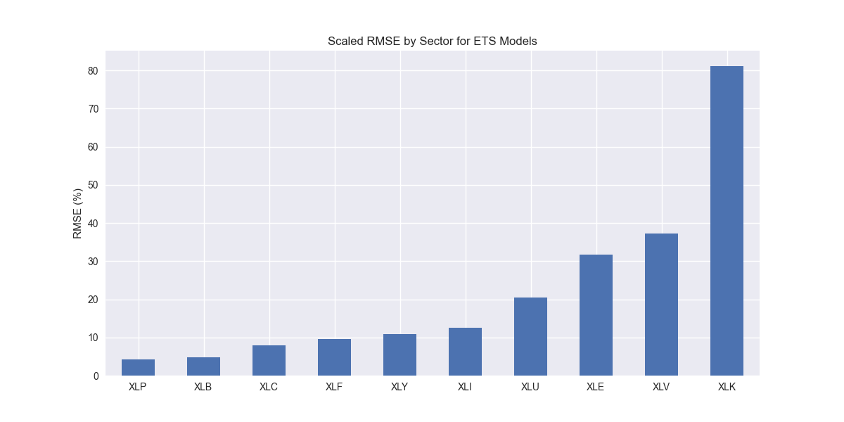
Nothing out of the ordinary. Some of the sectors trade places compared to the ETWS model, but we’ll leave that analysis for now. Let's compare to the benchmarks.

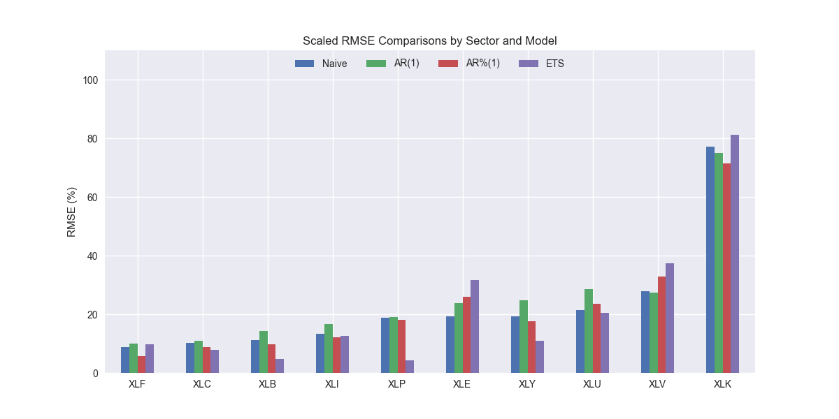
The ETS model appears better than the naive model at a 60/40 ratio. It's scaled RMSE is lower than the naive model for XLB, XLC, XLI, XLU, XLP, and XLY, the materials, communications, industrials, utilities, staples, and discretionary ETFs. For the remainder, it's worse. Let's confirm the aggregate performance below.

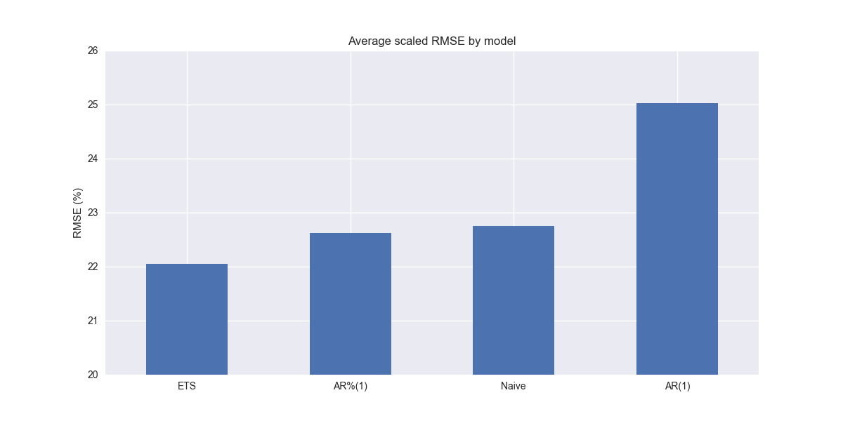
The ETS model does indeed outperform the naive and AR%(1) models. Comparing the above graph with the ETWS model graph from the last post one might be tempted to say it is slightly better. But the differences are in basis points. Nonetheless, in our next post we’ll compare the two to see if there are any major differences warranting preference of one over the other. Stay tuned!

Code below.

# Load packages
import numpy as np
import pandas as pd
from datetime import datetime, timedelta
import statsmodels.api as sm
import matplotlib.pyplot as plt
from matplotlib.ticker import FuncFormatter
import matplotlib as mpl
import pickle
from statsmodels.tsa.exponential_smoothing.ets import ETSModel

# Assign chart style
plt.style.use('seaborn-v0_8')
plt.rcParams["figure.figsize"] = (12,6)

# Handy functions
# Functions to load and save files
def save_dict_to_file(data, filename):
    with open(filename, 'wb') as f:
        pickle.dump(data, f)

def load_dict_from_file(filename):
    with open(filename, 'rb') as f:
        return pickle.load(f)

# Create functions for indexing
def create_index(series):
    if series.iloc[0] > 0:
        return series/series.iloc[0] * 100
    else:
        return (series - series.iloc[0])/-series.iloc[0] * 100

# Function for scaled RMSE
def get_rmse_scaled(series):
    return np.sqrt(np.mean((series['actual']-series['predicted'])**2))/np.mean(series['actual'])

# Function to flatten
def flatten_df(dataf: pd.DataFrame, group_name:str, cols:list) -> pd.DataFrame:
    df_grouped = dataf.groupby(group_name)[cols].agg(list)

    for col in cols:
        df_grouped[col] = df_grouped[col].apply(lambda x: np.concatenate(x))
    
    df_long = df_grouped.apply(pd.Series.explode).reset_index()

    return df_long

# Symbols used
etf_symbols = ['XLF', 'XLI', 'XLE', 'XLK', 'XLV', 'XLY', 'XLP', 'XLB', 'XLU', 'XLC']

ticker_list = ["SHW", "LIN", "ECL", "FCX", "VMC",
               "XOM", "CVX", "COP", "WMB", "SLB",
               "JPM", "V", "MA", "BAC", "GS",
               "CAT", "RTX", "DE", "UNP", "BA",
               "AAPL", "MSFT", "NVDA", "ORCL", "CRM",
               "COST", "WMT", "PG", "KO", "PEP",
               "NEE", "D", "DUK", "VST", "SRE",
               "LLY", "UNH", "JNJ", "PFE", "MRK",
               "AMZN", "SBUX", "HD", "BKNG", "MCD",
               "META", "GOOG", "NFLX", "T", "DIS"
]

xlb = ["SHW", "LIN", "ECL", "FCX", "VMC"]
xle = ["XOM", "CVX", "COP", "WMB", "SLB"]
xlf = ["JPM", "V", "MA", "BAC", "GS"]
xli = ["CAT", "RTX", "DE", "UNP", "BA"]
xlk = ["AAPL", "MSFT", "NVDA", "ORCL", "CRM"]
xlp = ["COST", "WMT", "PG", "KO", "PEP"]
xlu = ["NEE", "D", "DUK", "VST", "SRE"]
xlv = ["LLY", "UNH", "JNJ", "PFE", "MRK"]
xly = ["AMZN", "SBUX", "HD", "BKNG", "MCD"]
xlc = ["META", "GOOG", "NFLX", "T", "DIS"]

sectors = [xlf,  xli,  xle,  xlk, xlv,  xly, xlp, xlb, xlu, xlc]

# Sector dictionary
sector_dict = {symbol.lower(): tickers for symbol, tickers in zip(etf_symbols, sectors)}
sector_map = {ticker.lower(): symbol for symbol, tickers in zip(etf_symbols, sectors) for ticker in tickers}

# Load data from disk
# See Code Walk-Throughs for how we built the data set
df_sector_dict = load_dict_from_file("path/to/data/simfin_df_rev_dict.pkl")

# Clean dataframes
df_rev_index_dict = {}
for key in sector_dict:
    temp_df = df_sector_dict[key].copy()
    col_1 = temp_df.columns[0]
    temp_df = temp_df[[col_1] + [x for x in temp_df.columns if 'revenue' in x]]
    temp_df.columns = ['date'] + [x.replace('revenue_', '').lower() for x in temp_df.columns[1:]]
    temp_idx = temp_df.copy()
    temp_idx[[x for x in temp_idx if 'date' not in x]] = temp_idx[[x for x in temp_idx if 'date' not in x]].apply(create_index)
    df_rev_index_dict[key] = temp_idx

# Create train/test dataframes
df_rev_train_dict = {}
df_rev_chg_train_dict = {}
df_rev_test_dict = {}
for key in df_rev_index_dict:
    # Create ticker list
    tickers = [x.lower() for x in sector_dict[key]]
    
    # Create dataframe fo all
    df_out = df_rev_index_dict[key]

    # Base train df
    df_train = df_out.loc[df_out['date'] < "2023-01-01"].copy()
    df_rev_train_dict[key] = df_train
    
    # Chang train df
    df_train_chg = df_train.copy()
    df_train_chg[tickers] = df_train_chg[tickers].apply(lambda x: np.log(x).diff())
    df_train_chg = df_train_chg.dropna()
    df_rev_chg_train_dict[key] = df_train_chg

    # Test df
    df_rev_test_dict[key] = df_out.loc[df_out['date'] >= "2023-01-01"]

# Create ETS models
ets_models = {}
for key in df_rev_chg_train_dict:
    tickers = [x.lower() for x in sector_dict[key]]
    df_train = df_rev_train_dict[key]
    ets_models[key] = {}
    for ticker in tickers:
        try: 
            model = ETSModel(
                df_train[ticker],
                error='add',          # 'add' or 'mul'
                trend='add',          # 'add', 'mul', or None
                seasonal='add',       # 'add', 'mul', or None
                seasonal_periods=4
            ).fit(disp=False)
 
        except ValueError as e:
            print(f"{ticker} fails due to {e}")

        ets_models[key][ticker] = model

ets_err_df = pd.DataFrame(columns = ['sector', 'ticker', 'actual', 'predicted'])
count = 0
# forecast_horizon = np.arange(16,19)
for key in ets_models:
    for ticker in ets_models[key]:
        
        # Forecast the next 4 quarters
        y_pred = ets_models[key][ticker].get_prediction(start=16, end=19).predicted_mean
        y_act = df_rev_test_dict[key][ticker].values

        ets_err_df.loc[count] = [key.upper(), ticker, y_act, y_pred]
        count += 1

for ticker in ets_err_df['ticker'].to_list():
    actual = ets_err_df.loc[ets_err_df['ticker']==ticker, 'actual'].values[0]
    predicted = ets_err_df.loc[ets_err_df['ticker']==ticker, 'predicted'].values[0]
    rmse = np.sqrt(np.mean((actual - predicted)**2))
    rmse_scaled = rmse/actual.mean()
    ets_err_df.loc[ets_err_df['ticker']==ticker, 'rmse'] = rmse
    ets_err_df.loc[ets_err_df['ticker']==ticker, 'rmse_scaled'] = rmse_scaled
  
# Clean and flatten ar_err_df
ets_df_long = flatten_df(ets_err_df, 'sector', ['actual', 'predicted'])

# Graph scaled RMSE by sector
(ets_df_long.groupby('sector')[['actual', 'predicted']].apply(get_rmse_scaled).sort_values(ascending=True)*100).plot(kind='bar', rot=0)
plt.xlabel('')
plt.ylabel('RMSE (%)')
plt.title('Scaled RMSE by Sector for ETS Models')
plt.show()

# Get benchmarks
comp_df = pd.read_pickle("path/to/data/comp_new_df.pkl")
ets = ets_df_long.groupby('sector')[['actual', 'predicted']].apply(get_rmse_scaled).reset_index().rename(columns={0:'ets'})
comp_df = comp_df.merge(ets, how="left", on='sector')
comp_df.iloc[:, 1:].mean()*100

# Plot RMSE by sector and model  
(comp_df.set_index('sector')[['naive', 'lr', 'chg','ets']].sort_values('naive')*100).plot(kind='bar', rot=0)
plt.xlabel('')
plt.ylabel('RMSE (%)')
plt.ylim(0, 110)
plt.legend(['Naive', 'AR(1)', 'AR%(1)', 'ETS'], loc='upper center', ncol=4)
plt.title('Scaled RMSE Comparisons by Sector and Model')
plt.show()

# Plot Average performance
x_lab_dict = {'naive': 'Naive', 'lr': 'AR(1)', 'chg': 'AR%(1)', 'ets':'ETS'}
x_labs = comp_df.iloc[:, 1:].mean().sort_values().index.to_list()

(comp_df.iloc[:, 1:].mean().sort_values()*100).plot(kind='bar', rot=0)
plt.xticks(np.arange(4), [x_lab_dict[x] for x in x_labs])
plt.ylabel('RMSE (%)')
plt.ylim(20,26)
plt.title('Average scaled RMSE by model')
plt.savefig("hello_world/images/day_18_avg_rmse.png")
plt.show()

# Comparisons
comp_df.loc[comp_df['ets']<comp_df['naive'], 'sector']
comp_df.loc[comp_df['ets']>comp_df['naive'], 'sector']