BOTW 3: Rolling a pair

Using rolling regressions improves the OIH/USO pairs trade

Pairs trading is a popular approach in quant finance, coming in all sorts of flavors—from simple correlation and cointegration to all forms of statistical arbitrage in different timeframes down to the second. The concept is relatively straightforward. There exists some relationship between two or more assets that obtains over a set timeframe. The strength of this relationship implies that when the underlying assets exceed some threshold, they will reverse direction, from which one can make money.

Simplistically, if asset A has gone up 5% while asset B has only gone up 2%, but usually goes up 4%, then one goes long asset B and shorts asset A. If the opposite happens, one reverses the trade. Now, it can be more a lot more complicated than this and one can add a bunch of bells and whistles, but that is the gist. In his book, Quantitative Trading, Dr. Ernest P. Chan has some nice examples. Indeed, he uses the classic (pun intended) Coke vs. Pepsi pair as one. But another interesting one is GLD vs. GDX, the gold vs. the gold miner ETFs. There are, of course, other famous examples like GM vs Ford, Exxon vs. Chevron, and Blackberry vs. Nokia, or maybe that was just a flat out short Blackberry.

While these relationships can have intuitive appeal, equity research analysts are likely to offer fundamental reasons why such relationships would change before they show up in the statistical relationships. Pepsi getting into the snack food business is a good example. In other words, when the underlying market exposures change, the statistical relationships should change too. If you believe in the efficient market hypothesis, that should be instantaneous. We're not so sure.

The key point is that statistical relationships are backward looking. On the other side of the coin, analysts who are not using statistical models, but using domain expertise and fundamental research along with the need to remain (somewhat) market neutral will recommend pairs trades that might not be supported by historical relationships. For example, long Home Depot / short Lowe's might be a typical trade that has worked well. (This is entirely for informational purposes. Not an investment recommendation!) But if an analyst has learned through channel checks that Lowe's revamped paint offerings are generating more foot traffic and gaining traction with pro painters, she might recommend the opposite trade until the market has figured out the same thing or it shows up in results.

Recommending such a trade would require lots of domain knowledge, due diligence, and a substantial amount of intuition around sentiment/expectations. We don’t have such knowledge, at least in regard to hardlines home improvement, so we’ll have let the data dictate our trade.

Let's set up a typical pairs trade and see if we can improve upon it. In the book, Dr. Chan uses GLD vs. GDX and KO vs. PEP. We'll show something a little different. USO vs. OIH. OIH is the Oil Services ETF, whose members include companies like Schlumberger, Baker Hughes, and Haliburton; in other words, companies that provide the machinery and services to extract oil and other fossil fuels. The idea here is that the price of oil drives the desire to drill which drives the demand for oil services. We'll split the data into a train and test period and then run a linear regression with USO as the x-variable and OIH as the y, assuming a zero intercept¹. We then use the coefficient as the amount by which to short USO against OIH. When the spread is positive, OIH is performing better than USO and vice versa. Let's see what the spread looks like in sample.

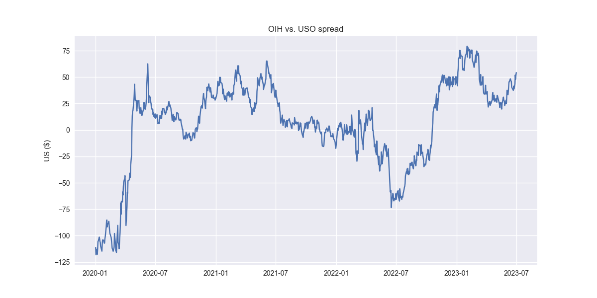
Now, we'll construct a trading strategy that says when the spread is below -1 standard deviation go long and reverse to short when it's above 1 standard deviation. That looks like the following in the training set.

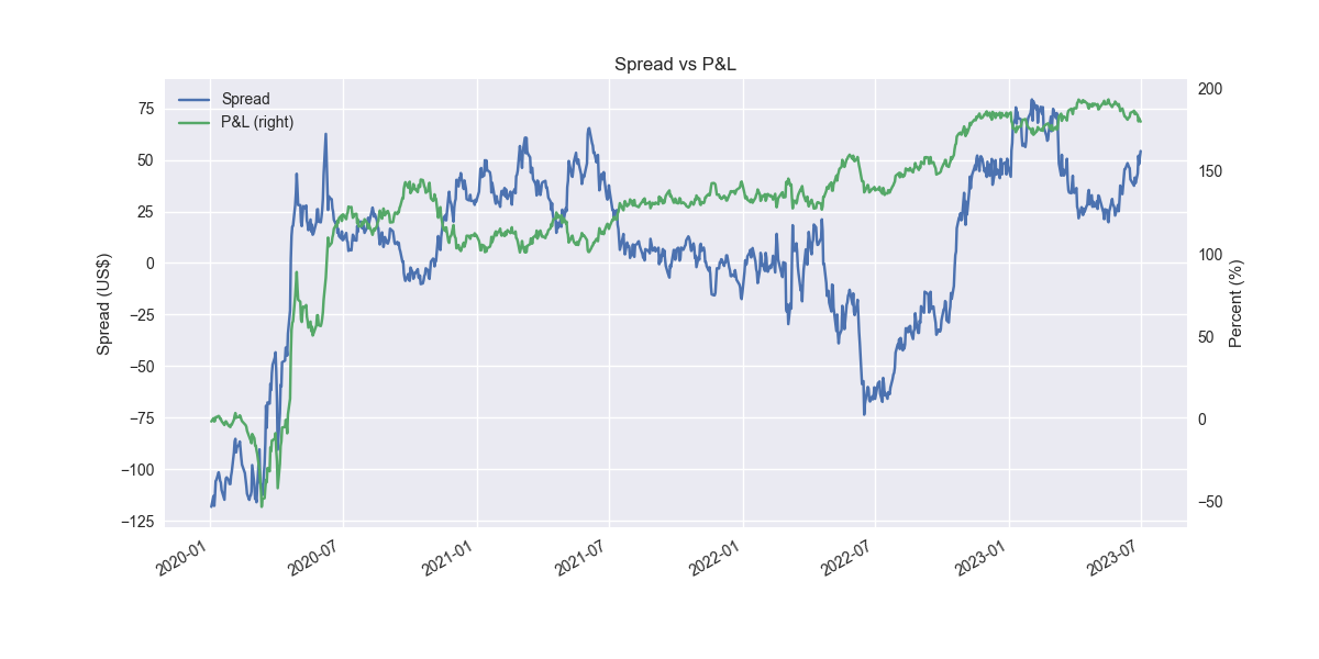
Pretty amazing. But clearly snooping going on. Here it is out-of-sample.

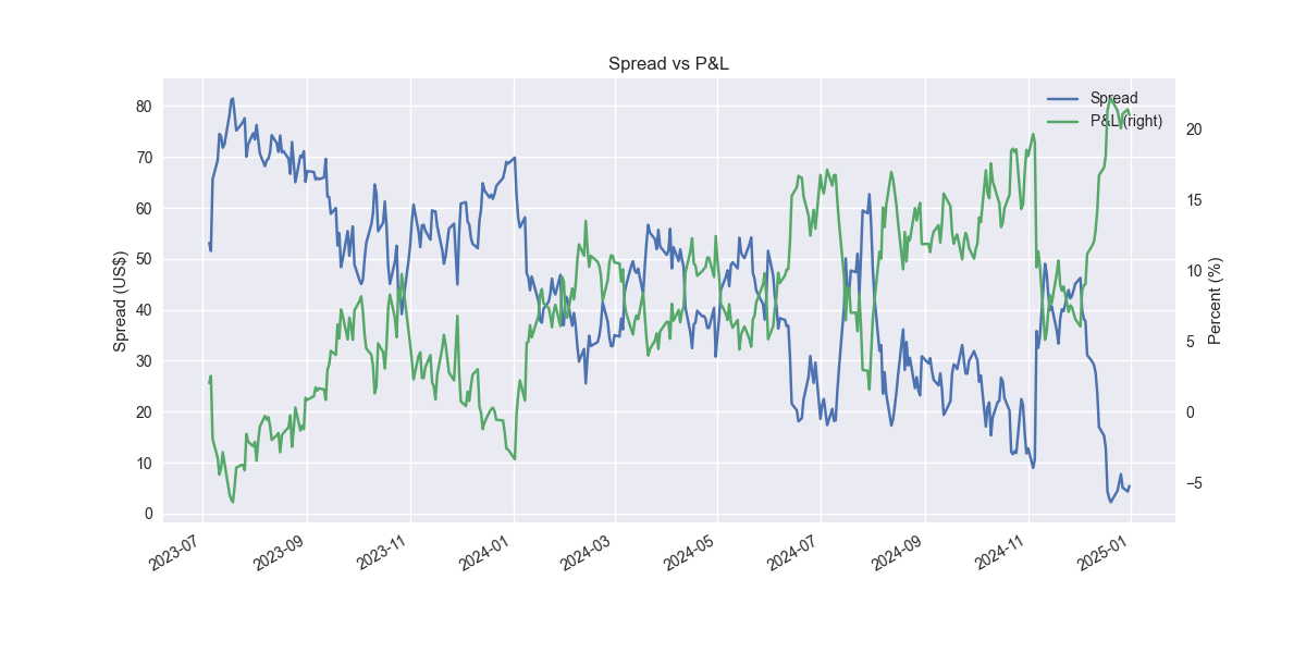
Not so great and pretty shaky. Let’s refine. The issue is that we're assuming the relationship we found on the training set will hold for the out-of-sample test. Markets aren't that stable, especially when dealing with daily data. So we should accommodate that instability by allowing the relationship to change. An easy way to do that is by simply running a rolling regression. Let's use a 60-day window, which equates to about three months of trading days. For brevity, we won't show the training set, just the out-of-sample test.

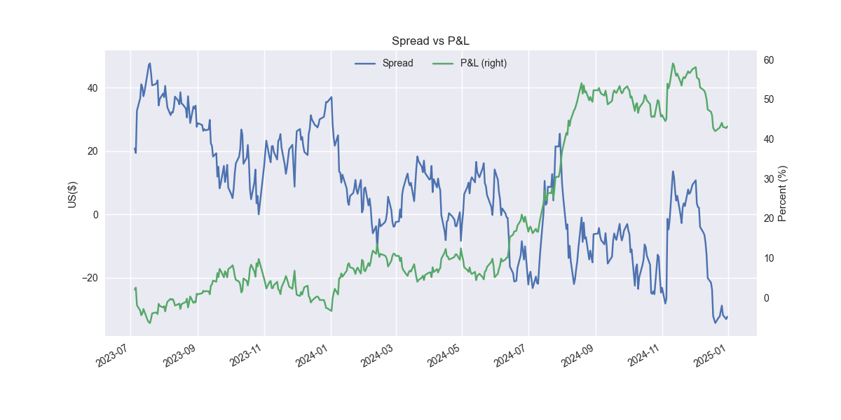
Not bad. One can see that the cumulative performance is better for the rolling model at 43% vs. 21% for the static model. Importantly, the Sharpe ratio of the rolling model is 1.19, more than 60 points better than the static model's Sharpe of 0.58. One should note that we don't actually roll in the test set, carrying forward that last model's output instead. Thus, performance could improve from here, but we won’t know until we test.

The key takeaway is that employing a modest refinement to the pairs trading strategy yields a nice improvement. We could add more refinements like cross-validating the lookback window or using a sign forecast as a filter. And the success we saw with OIH vs. USO might simply have been random. Rolling regression might not work with other pairs trades. All good observations that we'll save that for another post. Stay tuned!

Code below.

# Import packages
import numpy as np
import pandas as pd
import matplotlib.pyplot as plt
import statsmodels.api as sm
from statsmodels.tsa.stattools import coint
from statsmodels.regression.rolling import RollingOLS
import yfinance as yf

plt.style.use('seaborn-v0_8')
plt.rcParams['figure.figsize'] = (12,6)

# Functions   
def get_data(x_ticker, y_ticker, start_date, end_date):
    if type(x_ticker) == 'list':
        tickers = x_ticker + [y_ticker]
    else:
        tickers = [x_ticker, y_ticker]

    return yf.download(tickers, start_date, end_date)['Close'] #type: ignore

    
def get_returns(dataf):
    return dataf.apply(lambda x: np.log(x/x.shift()))


def get_diff(dataf):
    return dataf.diff()


def get_train_test(dataf, period=0.7):
    train_set = np.arange(0, int(dataf.shape[0]*period))
    test_set = np.arange(train_set.shape[0], dataf.shape[0])
    return train_set, test_set


def get_coint(dataf, y_ticker, x_ticker, period_set, print_out=True, dat_out=False):
    coint_t, p_value, _ = coint(dataf[y_ticker].iloc[period_set], dataf[x_ticker].iloc[period_set])
    if print_out:
        print(f'P-value is : {p_value:0.3f}')
    if dat_out:
        return coint_t, p_value
    

def get_hedgeratio(dataf, x_ticker, y_ticker, period_set, rolling=True, window=60):

    df = dataf.copy()

    if rolling:
        model = RollingOLS(df.loc[:, y_ticker].iloc[period_set], 
                            df.loc[:, x_ticker].iloc[period_set],
                            window=window)
    else:
        model = sm.OLS(df.loc[:, y_ticker].iloc[period_set], df.loc[:, x_ticker].iloc[period_set])       
    
    results = model.fit()
    hr = results.params.values

    if rolling:
        n_nans = len(dataf) - hr.shape[0]
        nan_arr = np.full((n_nans, 1), np.nan)
        hr = pd.DataFrame(np.vstack([hr, nan_arr]), index=dataf.index, columns=[x_ticker])
        hr = hr.ffill()

    return hr


def get_spread(dataf, x_ticker, y_ticker, hedge_ratio, type='regression', rolling=True):
    
    if type == 'regression':    
        if rolling:
            spread = dataf.loc[:,y_ticker] - hedge_ratio[x_ticker]*dataf.loc[:,x_ticker]
            # spread = dataf.loc[:,x_ticker] - hedge_ratio[x_ticker]*dataf.loc[:,y_ticker]
        else:
            spread = dataf.loc[:,y_ticker] - hedge_ratio[0]*dataf.loc[:,x_ticker]
            # spread = dataf.loc[:,x_ticker] - hedge_ratio[0]*dataf.loc[:,y_ticker]
    else:
        spread = dataf.loc[:,y_ticker] - dataf.loc[:,x_ticker]
        # spread = dataf.loc[:,x_ticker] - dataf.loc[:,y_ticker]

    return spread


def plot_spread(spread, x_ticker, y_ticker, period_set):
    if type(x_ticker) == 'list':
        x_ticker = " & ".join([x for x in x_ticker])

    plt.plot(spread[period_set])
    plt.title(f"{y_ticker} vs. {x_ticker} spread")
    plt.ylabel("US ($)")
    plt.show()
    

def get_signals(dataf, spread, x_ticker, y_ticker, period_set, enter=2.0, exit=1.0):

    spreadMean = np.mean(spread.iloc[period_set])
    spreadVol = np.std(spread.iloc[period_set])

    signals_df = dataf.copy()

    signals_df['zscore'] = (spread - spreadMean)/spreadVol

    signals_df[f"pos_{y_ticker}_long"] = np.nan
    signals_df[f"pos_{y_ticker}_short"] = np.nan

    if type(x_ticker) == "list":
        for ticker in x_ticker:
            signals_df[f"pos_{ticker}_long"] = np.nan
            signals_df[f"pos_{ticker}_short"] = np.nan
    else:
        signals_df[f"pos_{x_ticker}_long"] = np.nan
        signals_df[f"pos_{x_ticker}_short"] = np.nan

    if type(x_ticker) == "list":
        pass
    else:
        signals_df.loc[signals_df.zscore>=enter, (f"pos_{y_ticker}_short", f"pos_{x_ticker}_short")]=[-1, 1] # Short spread
        signals_df.loc[signals_df.zscore<=-enter, (f"pos_{y_ticker}_long", f"pos_{x_ticker}_long")]=[1, -1] # Buy spread
        signals_df.loc[signals_df.zscore<=exit, (f"pos_{y_ticker}_short", f"pos_{x_ticker}_short")]=0 # Exit short spread
        signals_df.loc[signals_df.zscore>=-exit, (f"pos_{y_ticker}_long", f"pos_{x_ticker}_long")]=0 # Exit long spread

    signals_df.ffill(inplace=True)

    return signals_df


def get_positions(signals_df, x_ticker, y_ticker):
    if type(x_ticker) == 'list':
        pass
    else:
        positions_long=signals_df.loc[:, (f"pos_{y_ticker}_long", f"pos_{x_ticker}_long")].copy()
        positions_short=signals_df.loc[:, (f"pos_{y_ticker}_short", f"pos_{x_ticker}_short")].copy()
        positions=np.array(positions_long)+np.array(positions_short)
        positions=pd.DataFrame(positions)
    
    return positions

def get_pnl(positions):
    pnl = (np.array(positions.shift())*np.array(returns)).sum(axis=1)
    return pnl


def get_sharpe(pnl, period_set, period=252):
    with np.errstate(invalid='ignore'):
        out = np.sqrt(period)*np.mean(pnl[period_set[1:]])/np.std(pnl[period_set[1:]])
        if str(out) == 'nan':
            return 0
        else:
            return out

def get_cumul_pnl(pnl, period_set):
    return pnl[period_set[1:]].cumsum()[-1]


def plot_pnl(spread, pnl, period_set):
    ax = pd.DataFrame(spread[period_set[1:]], columns=['Spread']).plot(ylabel='US($)')
    
    ax2 = (pd.DataFrame(pnl[period_set[1:]], 
                    index=spread.index[period_set[1:]],
                    columns=['P&L']).cumsum()*100).plot(secondary_y=True, ax=ax)
    

    ax.set_xlabel("")
    ax.set_ylabel('Spread (US$)')
    ax2.set_ylabel('Percent (%)')
    plt.title('Spread vs P&L')
    plt.show()

# Parameters
x_ticker = 'USO'
y_ticker = 'OIH'
start_date = '2020-01-01' 
end_date = '2025-01-01'

# Get data
data = get_data(x_ticker, y_ticker, start_date, end_date)
train, test = get_train_test(data)

# Get hedge ratios
hr_static = get_hedgeratio(data, x_ticker, y_ticker, train, rolling=False)
hr_roll = get_hedgeratio(data, x_ticker, y_ticker, train)

# Get spreads
spread_static = get_spread(data, x_ticker, y_ticker, hr_static, rolling=False)
spread_roll = get_spread(data, x_ticker, y_ticker, hr_roll)

# Plot spreads
plot_spread(spread_static, x_ticker, y_ticker, train)
plot_spread(spread_static, x_ticker, y_ticker, test)

plot_spread(spread_roll, x_ticker, y_ticker, train)
plot_spread(spread_roll, x_ticker, y_ticker, test)

# Get returns
returns = get_returns(data)

# Construct static signal
signals_static = get_signals(data, spread_static, x_ticker, y_ticker, train, enter=1, exit=-1)
positions_static = get_positions(signals_static, x_ticker, y_ticker)
pnl_static = get_pnl(positions_static)
plot_pnl(spread_static, pnl_static, train)
plot_pnl(spread_static, pnl_static, test)

# Construct rolling signal
signals_roll = get_signals(data, spread_roll, x_ticker, y_ticker, train, enter=1, exit=-1)
positions_roll = get_positions(signals_roll, x_ticker, y_ticker)
pnl_roll = get_pnl(positions_roll)
plot_pnl(spread_roll, pnl_roll, train)
plot_pnl(spread_roll, pnl_roll, test)

# Calculate performance statistics
static_cumul = get_cumul_pnl(pnl_static, test)
roll_cumul = get_cumul_pnl(pnl_roll, test)
print(static_cumul)
print(roll_cumul)

static_sharpe = get_sharpe(pnl_static, test)
roll_sharpe = get_sharpe(pnl_roll, test)
print(static_sharpe)
print(roll_sharpe)
print(roll_sharpe - static_sharpe)

1. Using a zero intercept assumes that there is no reason one stock or ETF should outperform the other. That is also why we subtract the x-variable times its coefficient from the y-variable to obtain the zero value. When the spread drifts two far from that value, an arbitrage opportunity emerges.