HFW 1: Naïveté

We discuss the logic of the dataset and establish a naïve benchmark

In our last post, Hello Forecasting World!, (or HFW 0), we established the motivation for this series: test the main time series algorithms on their predictive accuracy to forecast revenues. Of course, the devil is in the details for how we plan to do this. We need a fairly representative dataset that captures different industries, economic exposures, and reporting conventions. The dataset also needs to be manageable enough so that the reader can do this at home without having to pay for a data stream or API feed. It would be easy enough to connect to Factset or Bloomberg and pull the data. But that would require some beaucoup bucks for the privilege and ease. That doesn't work for the philosophy of this blog, which is to ensure that most results are reproducible (within reason of course!). The process to do this was actually more involved than we expected, having had to experiment with AlphaVantage, SimFin, Tiingo, and Yahoo! We detail how we built the dataset in Code Walk-Throughs. For now, we'll summarize the process.

Why do we want to capture different industries, economic exposures, and reporting conventions? Logically, there are likely to be some algorithms that are randomly better suited to forecasting Caterpillar's revenues as opposed to Pfizer's. Not accounting for that would—knowingly or not—yield biased results. Additionally, a buyside fundamental analyst would likely need to forecast revenues for a range of industries and companies, so it would behoove him or her to know if there is a performant, general purpose algorithm that can be applied across the board. The constraints to all of this are free data, a sufficiently long period, and manageable size.

We chose the main S&P 500 sectors, as represented by the Select SPDR®. Within each sector we chose five stocks from the top ten holdings. We started with the top five, but if the data wasn't available or plain wrong, we moved down the list. For the API, we eventually settled on using SimFin. It didn't have the longest time series, but it had the fewest errors. There was some missing data, but that had more to do with the feed, and we were able to correct those issues programmatically. Having spent years adjusting financial statement items from different data providers, believe us when we tell you it's an arduous task.

Having worked through all the APIs and wrangling, we settled on the five stocks from each of the following ETFs: XLF, XLI, XLE, XLK, XLV, XLY, XLP, XLB, XLU, and XLC. The dataset covers five years of quarterly data starting in 2019. We use 2019-2022 as the training period and then forecast the next four quarters for 2023. Some companies have non-calendar quarter ends—retail mostly. For those we associate the fiscal quarters with the calendar quarter in which a majority of the data falls. For example, for companies with a January 31st quarter end, we reposition the data to align with a December 31 quarter end. We also index the data to the beginning of the period for three reasons. First, it makes graphing the revenues of 50 companies easier to read. Second, it shows the relative differences in growth rates within and across industries. Finally, comparisons are just easier with everything is indexed to 100. We show the indexed training set below.

Now the trick is where do we start and what's the benchmark? Typically, the benchmark would be a naïve model in which we simply use the last value as the prediction. Since we're forecasting four steps ahead, that means the last value is repeated four times. We think this is actually too naïve. Even bad analysts would never do that. But we have to establish a baseline, even if it seems like it should be easy to beat. If public companies can issue guidance that they plan to beat, which everyone knows, and then they take a victory lap when they beat it, why can't we do the same! For now, we'll straight-line the forecasts. We then calculate individual stock and aggregate sector root mean-squared error (RMSE) and a scaled RMSE, which is RMSE divided by the average actual value. The scaled RMSE gives one a better perspective on how far the forecasts are in percentage terms. We show the scaled RMSE for each sector in the graph below.

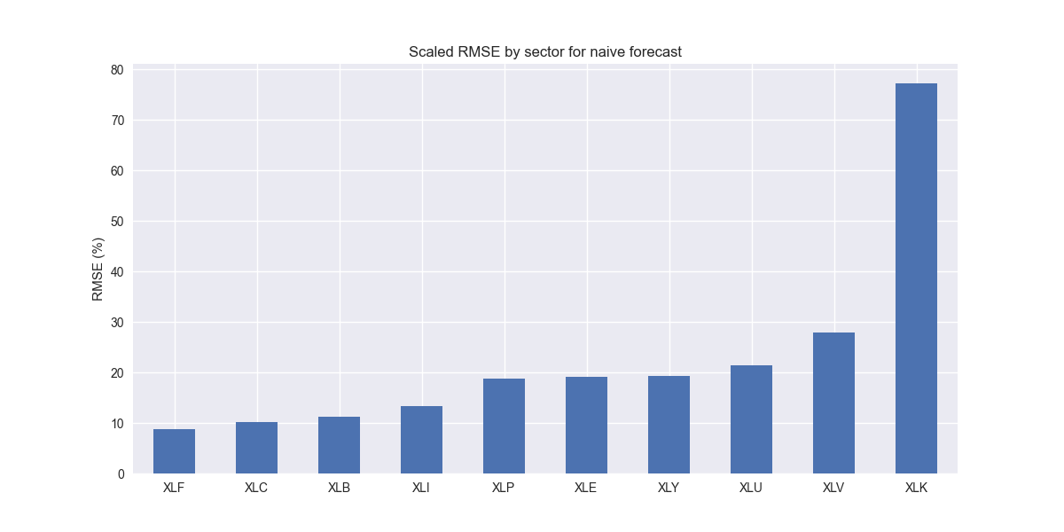
Excluding XLK, nothing jumps out here. Kind of like the CEO who said, "If we excluded the losses, this quarter would have been very profitable!" On XLK, the main cause for this outsized error is due to Nvidia, whose growth vs. the naïve forecast was 19%, 120%, 199%, and 262%. Enough said. In our next post, we'll set up our first forecast using an actual model. Stay tuned!

Code below:

# Load packages
import os
import requests
import pandas as pd
import numpy as np
from datetime import datetime, timedelta
import yfinance as yf
import statsmodels.api as sm
import matplotlib.pyplot as plt
from matplotlib.ticker import FuncFormatter
import matplotlib as mpl
import time
import re
import pickle

# Assign chart style
plt.style.use('seaborn-v0_8')
plt.rcParams["figure.figsize"] = (12,6)

# Functions to load files
# Load and save
def save_dict_to_file(data, filename):
    with open(filename, 'wb') as f:
        pickle.dump(data, f)

def load_dict_from_file(filename):
    with open(filename, 'rb') as f:
        return pickle.load(f)

# Symbols used
etf_symbols = ['XLF', 'XLI', 'XLE', 'XLK', 'XLV', 'XLY', 'XLP', 'XLB', 'XLU', 'XLC']

ticker_list = ["SHW", "LIN", "ECL", "FCX", "VMC",
               "XOM", "CVX", "COP", "WMB", "SLB",
               "JPM", "V", "MA", "BAC", "GS",
               "CAT", "RTX", "DE", "UNP", "BA",
               "AAPL", "MSFT", "NVDA", "ORCL", "CRM",
               "COST", "WMT", "PG", "KO", "PEP",
               "NEE", "D", "DUK", "VST", "SRE",
               "LLY", "UNH", "JNJ", "PFE", "MRK",
               "AMZN", "SBUX", "HD", "BKNG", "MCD",
               "META", "GOOG", "NFLX", "T", "DIS"
]

xlb = ["SHW", "LIN", "ECL", "FCX", "VMC"]
xle = ["XOM", "CVX", "COP", "WMB", "SLB"]
xlf = ["JPM", "V", "MA", "BAC", "GS"]
xli = ["CAT", "RTX", "DE", "UNP", "BA"]
xlk = ["AAPL", "MSFT", "NVDA", "ORCL", "CRM"]
xlp = ["COST", "WMT", "PG", "KO", "PEP"]
xlu = ["NEE", "D", "DUK", "VST", "SRE"]
xlv = ["LLY", "UNH", "JNJ", "PFE", "MRK"]
xly = ["AMZN", "SBUX", "HD", "BKNG", "MCD"]
xlc = ["META", "GOOG", "NFLX", "T", "DIS"]

sectors = [xlf,  xli,  xle,  xlk, xlv,  xly, xlp, xlb, xlu, xlc]

# Sector dictionary
sector_dict = {symbol.lower(): tickers for symbol, tickers in zip(etf_symbols, sectors)}

# Load data from disk
# See Code Walk-Throughs for how we built the data set
df_sector_dict = load_dict_from_file("hello_world/data/simfin_df_rev_dict.pkl")

# Create functions for indexing
def create_index(series):
    if series.iloc[0] > 0:
        return series/series.iloc[0] * 100
    else:
        return (series - series.iloc[0])/-series.iloc[0] * 100

# Clean dataframes
df_rev_index_dict = {}
for key in sector_dict:
    temp_df = df_sector_dict[key].copy()
    col_1 = temp_df.columns[0]
    temp_df = temp_df[[col_1] + [x for x in temp_df.columns if 'revenue' in x]]
    temp_df.columns = ['date'] + [x.replace('revenue_', '').lower() for x in temp_df.columns[1:]]
    temp_idx = temp_df.copy()
    temp_idx[[x for x in temp_idx if 'date' not in x]] = temp_idx[[x for x in temp_idx if 'date' not in x]].apply(create_index)
    df_rev_index_dict[key] = temp_idx

# Print dataframes for quick spot checking
for key in sector_dict:
    print(key)
    print(df_rev_index_dict[key].head())
    print('')

# Create train/test dataframes
df_rev_train_dict = {}
df_rev_test_dict = {}
for key in df_rev_index_dict:
    df_out = df_rev_index_dict[key]
    df_rev_train_dict[key] = df_out.loc[df_out['date'] < "2023-01-01"]
    df_rev_test_dict[key] = df_out.loc[df_out['date'] >= "2023-01-01"]

# Plot dataframes
fig, axes = plt.subplots(3, 3, sharey=False, sharex=True, figsize=(14,8))

for idx, ax in enumerate(fig.axes):
    etf = etf_symbols[idx].lower()
    stocks = [x.lower() for x in sector_dict[etf.lower()]]

    df_plot = df_rev_train_dict[etf]
    ax.plot(df_plot['date'], df_plot[stocks])
    ax.set_xlabel('')
    ax.tick_params(axis='x', rotation=45)
    ax.legend([x.upper() for x in stocks], fontsize=6, loc='upper left')
    if idx  == 3:
        ax.set_ylabel("Index")
    ax.yaxis.set_major_formatter(FuncFormatter(lambda x, p: f'{int(x):,}'))
    ax.set_title(etf.upper())

plt.tight_layout()
# plt.savefig('hello_world/images/indexed_rev.png')
plt.show()

# Create naive forecast
rmse_naive = []
for etf in etf_symbols:
    # Create forecast df
    fcst = df_rev_train_dict[etf.lower()].copy()
    cols = [x.lower() for x in sector_dict[etf.lower()]]
    # fcst[cols] = fcst[cols].apply(lambda x: np.log(x/x.shift(4)))

    # Get actuals and predicted
    actual =  df_rev_test_dict[etf.lower()].copy()
    predicted = fcst.loc[fcst.iloc[[-1]].index.repeat(4), cols]

    # Calculate rmse
    rmse_comp = np.sqrt(np.mean((actual.iloc[:,1:].T.values - predicted.T.values)**2, axis=1))
    rmse_all = np.sqrt(np.mean((actual.iloc[:,1:].T.values - predicted.T.values)**2))
    rmse = np.append(rmse_comp, rmse_all)

    # Calculate means
    avg = actual.iloc[:, 1:].mean().values
    avg_all = actual.iloc[:, 1:].values.flatten().mean()
    mean_all = np.append(avg,avg_all)

    # Create rmse dataframe
    names = cols + [f'{etf.lower()}_all']
    temp_df = pd.DataFrame(zip(names, rmse, mean_all), columns=['ticker','rmse', 'avg'])
    temp_df['rmse_scaled'] = temp_df['rmse']/temp_df['avg']
    temp_df['sector'] = etf
    rmse_naive.append(temp_df)

df_naive = pd.concat([x for x in rmse_naive], axis=0).reset_index(drop=True)
print(df_naive)

((df_naive.loc[df_naive['ticker'].isin([f"{x.lower()}_all" for x in etf_symbols]), 
             ['sector','rmse_scaled']]
             .set_index('sector')*100)
.sort_values('rmse_scaled')).plot(kind='bar', rot=0)
plt.xlabel('')
plt.ylabel('RMSE (%)')
plt.legend('')
plt.title('Scaled RMSE by sector for naive forecast')
# plt.savefig("hello_world/images/day_2_naive_sector_rmse.png")
plt.show()

# Why is XLK so poor? NVDA's explosive growth
print(df_rev_test_dict['xlk']['nvda'].div(df_rev_train_dict['xlk'].iloc[-1, 3])-1)