HFW 13: ARCH Complex

A basic ARCH model performs better than most of the previous models, but is modestly worse than the naïve and autoregressive growth rate models

The day has finally arrived to tackle heteroskedasticity. What? Multisyllabic or not, the concept is easier to understand than the word is to pronounce. As we've noted before, when you build a model, you'll typically want to investigate the residuals (or error terms depending on your school of thought). Such investigation can reveal whether they're random—evenly distributed around zero—or not—clustering, widening, narrowing, or other shapes. When your error terms are not random, then the model is not well-specified, which means you can't really trust its estimates.

If the error terms aren't random, then they probably exhibit non-constant variance. In other words, they form patterns like we described above. That means they exhibit heteroskedasticity. When the data are not time series, there are ways to deal with this heteroskedasticity. But time series are their own animals, often exhibiting serial correlation (e.g., autoregression). This frequently results in the error terms also exhibiting serial correlation. In other words, the size of the error in one period is related to the size in another. If that is the case, then one can use an autoregressive conditional heteroskedasticity (ARCH) model.

Beside the statistical reasons discussed above, the intuition behind the model is that time series exhibit time-varying volatility. What is that? Every market observer already knows. There are calm markets and there are volatile ones. That change from calm to volatile and back again is time-varying volatility. By modeling volatility as depending on past errors (often called shocks), one can embed some sort view about future volatility. And before we forget, the reason it's called conditional is that one of the model's assumptions is that the variance at time t, is based (e.g., conditioned) on the information prior to time t.

While this all sounds great in theory, there are few assumptions that one should be aware of. In its basic form, an ARCH model assumes that returns at time t are based on the mean returns of the prior periods plus an error term. That really doesn't exist for company revenues, stock prices, or anything with a trend, as in our dataset. But we'll use this base case for our first pass at the model.

Now that we've provided an all too cursory background on ARCH models, we can implement one to see how they perform relative to our benchmarks. Let's go!

We jump straight into the scaled root mean-squared error graph, which should be all too familiar by now.

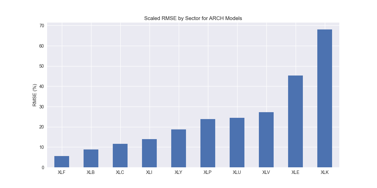
Nothing unusual here. Let's compare to the benchmarks.

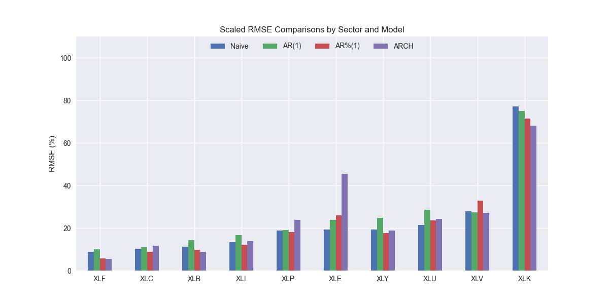
Interestingly, the ARCH model performs better than the naïve on XLF, XLB, XLK, XLV, and XLY. It performs worse on the others, XLE most notably. Thus far, the ARCH model performs the best on XLK compared to all others discussed to date; showing that some models are particularly well specified for certain sectors. While the ARCH model has pretty good performance in general, it does not beat the naïve or AR%(1) models, as shown in the graph below. That said, differences are small.

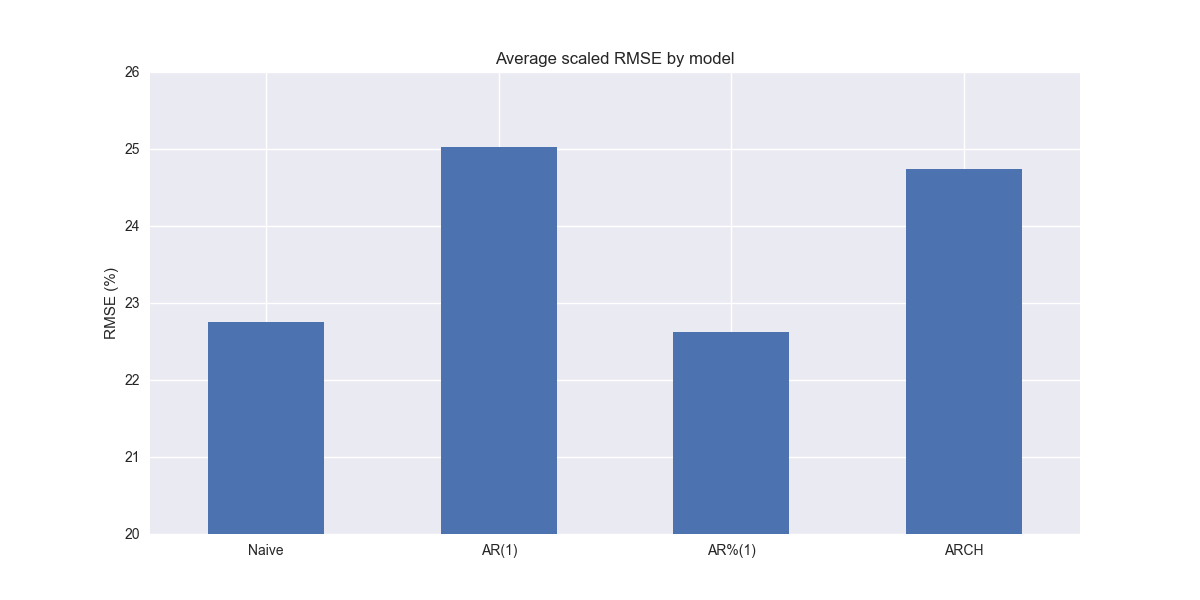
Recall that in its basic form, the ARCH model assumes returns will approximate the average value of the periods on which the model has been conditioned. That begs the question of how it performs relative to the average growth rate model we discussed back in Hello Forecasting World 10. While we don't show it here, the average growth rate model had about 1% point lower scaled RMSE on average than the ARCH model. This is probably too small to conclude much. But possible reasons for the better performance might be due to lack of sufficient volatility clustering and the limited amount of data, which can lead to overfitting.

Whatever the case, in the following posts will be experimenting with tweaking some of the ARCH model's parameters to see if we can improve performance as well as introducing GARCH, which includes lag variance terms in the model. More on that later. Stay tuned!

Code below.

# Load packages
import numpy as np
import pandas as pd
from datetime import datetime, timedelta
import statsmodels.api as sm
import matplotlib.pyplot as plt
from matplotlib.ticker import FuncFormatter
import matplotlib as mpl
import pickle
from arch import arch_model

# Assign chart style
plt.style.use('seaborn-v0_8')
plt.rcParams["figure.figsize"] = (12,6)

# Handy functions
# Functions to load and save files
def save_dict_to_file(data, filename):
    with open(filename, 'wb') as f:
        pickle.dump(data, f)

def load_dict_from_file(filename):
    with open(filename, 'rb') as f:
        return pickle.load(f)

# Create functions for indexing
def create_index(series):
    if series.iloc[0] > 0:
        return series/series.iloc[0] * 100
    else:
        return (series - series.iloc[0])/-series.iloc[0] * 100

# Function for scaled RMSE
def get_rmse_scaled(series):
    return np.sqrt(np.mean((series['actual']-series['predicted'])**2))/np.mean(series['actual'])

# Function to flatten
def flatten_df(dataf: pd.DataFrame, group_name:str, cols:list) -> pd.DataFrame:
    df_grouped = dataf.groupby(group_name)[cols].agg(list)

    for col in cols:
        df_grouped[col] = df_grouped[col].apply(lambda x: np.concatenate(x))
    
    df_long = df_grouped.apply(pd.Series.explode).reset_index()

    return df_long

# Symbols used
etf_symbols = ['XLF', 'XLI', 'XLE', 'XLK', 'XLV', 'XLY', 'XLP', 'XLB', 'XLU', 'XLC']

ticker_list = ["SHW", "LIN", "ECL", "FCX", "VMC",
               "XOM", "CVX", "COP", "WMB", "SLB",
               "JPM", "V", "MA", "BAC", "GS",
               "CAT", "RTX", "DE", "UNP", "BA",
               "AAPL", "MSFT", "NVDA", "ORCL", "CRM",
               "COST", "WMT", "PG", "KO", "PEP",
               "NEE", "D", "DUK", "VST", "SRE",
               "LLY", "UNH", "JNJ", "PFE", "MRK",
               "AMZN", "SBUX", "HD", "BKNG", "MCD",
               "META", "GOOG", "NFLX", "T", "DIS"
]

xlb = ["SHW", "LIN", "ECL", "FCX", "VMC"]
xle = ["XOM", "CVX", "COP", "WMB", "SLB"]
xlf = ["JPM", "V", "MA", "BAC", "GS"]
xli = ["CAT", "RTX", "DE", "UNP", "BA"]
xlk = ["AAPL", "MSFT", "NVDA", "ORCL", "CRM"]
xlp = ["COST", "WMT", "PG", "KO", "PEP"]
xlu = ["NEE", "D", "DUK", "VST", "SRE"]
xlv = ["LLY", "UNH", "JNJ", "PFE", "MRK"]
xly = ["AMZN", "SBUX", "HD", "BKNG", "MCD"]
xlc = ["META", "GOOG", "NFLX", "T", "DIS"]

sectors = [xlf,  xli,  xle,  xlk, xlv,  xly, xlp, xlb, xlu, xlc]

# Sector dictionary
sector_dict = {symbol.lower(): tickers for symbol, tickers in zip(etf_symbols, sectors)}
sector_map = {ticker.lower(): symbol for symbol, tickers in zip(etf_symbols, sectors) for ticker in tickers}

# Load data from disk
# See Code Walk-Throughs for how we built the data set
df_sector_dict = load_dict_from_file("path/to/data/simfin_df_rev_dict.pkl")

# Clean dataframes
df_rev_index_dict = {}
for key in sector_dict:
    temp_df = df_sector_dict[key].copy()
    col_1 = temp_df.columns[0]
    temp_df = temp_df[[col_1] + [x for x in temp_df.columns if 'revenue' in x]]
    temp_df.columns = ['date'] + [x.replace('revenue_', '').lower() for x in temp_df.columns[1:]]
    temp_idx = temp_df.copy()
    temp_idx[[x for x in temp_idx if 'date' not in x]] = temp_idx[[x for x in temp_idx if 'date' not in x]].apply(create_index)
    df_rev_index_dict[key] = temp_idx

# Create train/test dataframes
df_rev_train_dict = {}
df_rev_chg_train_dict = {}
df_rev_test_dict = {}
for key in df_rev_index_dict:
    # Create ticker list
    tickers = [x.lower() for x in sector_dict[key]]
    
    # Create dataframe fo all
    df_out = df_rev_index_dict[key]

    # Base train df
    df_train = df_out.loc[df_out['date'] < "2023-01-01"].copy()
    df_rev_train_dict[key] = df_train
    
    # Chang train df
    df_train_chg = df_train.copy()
    df_train_chg[tickers] = df_train_chg[tickers].apply(lambda x: np.log(x).diff())
    df_train_chg = df_train_chg.dropna()
    df_rev_chg_train_dict[key] = df_train_chg

    # Test df
    df_rev_test_dict[key] = df_out.loc[df_out['date'] >= "2023-01-01"]

arch_models = {}
for key in df_rev_chg_train_dict:
    tickers = [x.lower() for x in sector_dict[key]]
    df_train = df_rev_chg_train_dict[key]
    arch_models[key] = {}
    for ticker in tickers:
        try: 
            model = arch_model(df_train[ticker]*100, vol='ARCH', p=1).fit(disp="off")
        except ValueError as e:
            print(f"{ticker} fails due to {e}")

        arch_models[key][ticker] = model

arch_err_df = pd.DataFrame(columns = ['sector', 'ticker', 'actual', 'predicted'])
count = 0
for key in arch_models:
    for ticker in arch_models[key]:
        base_rev = df_rev_train_dict[key][ticker].iloc[-1]   
        mean_log_return = df_rev_chg_train_dict[key][ticker].mean()

        # Forecast the next 4 quarters' volatility
        forecast_horizon = 4
        arch_forecast = arch_models[key][ticker].forecast(horizon=forecast_horizon)
        forecast_mean = arch_forecast.mean

        # Convert log returns back to revenue levels
        y_pred = []
        for fcst in forecast_mean.values[0]:
            base_rev *= np.exp(fcst/100)
            y_pred.append(base_rev)

        y_act = df_rev_test_dict[key][ticker].values

        arch_err_df.loc[count] = [key.upper(), ticker, y_act, y_pred]
        count += 1

for ticker in arch_err_df['ticker'].to_list():
    actual = arch_err_df.loc[arch_err_df['ticker']==ticker, 'actual'].values[0]
    predicted = arch_err_df.loc[arch_err_df['ticker']==ticker, 'predicted'].values[0]
    rmse = np.sqrt(np.mean((actual - predicted)**2))
    rmse_scaled = rmse/actual.mean()
    arch_err_df.loc[arch_err_df['ticker']==ticker, 'rmse'] = rmse
    arch_err_df.loc[arch_err_df['ticker']==ticker, 'rmse_scaled'] = rmse_scaled
  
# Clean and flatten ar_err_df
arch_df_long = flatten_df(arch_err_df, 'sector', ['actual', 'predicted'])

# Graph scaled RMSE by sector
(arch_df_long.groupby('sector')[['actual', 'predicted']].apply(get_rmse_scaled).sort_values(ascending=True)*100).plot(kind='bar', rot=0)
plt.xlabel('')
plt.ylabel('RMSE (%)')
plt.title('Scaled RMSE by Sector for ARCH Models')
plt.show()

comp_df = pd.read_pickle("hello_world/data/comp_new_df.pkl")
arch = arch_df_long.groupby('sector')[['actual', 'predicted']].apply(get_rmse_scaled).reset_index().rename(columns={0:'arch'})
comp_df = comp_df.merge(arch, how="left", on='sector')

# Plot RMSE by sector and model
(comp_df.set_index('sector')[['naive', 'lr', 'chg','arch']].sort_values('naive')*100).plot(kind='bar', rot=0)
plt.xlabel('')
plt.ylabel('RMSE (%)')
plt.ylim(0, 110)
plt.legend(['Naive', 'AR(1)', 'AR%(1)', 'ARCH'], loc='upper center', ncol=4)
plt.title('Scaled RMSE Comparisons by Sector and Model')
plt.show()

(comp_df.iloc[:, 1:].mean()*100).plot(kind='bar', rot=0)
plt.xticks(np.arange(4), ['Naive', 'AR(1)', 'AR%(1)', 'ARCH'])
plt.ylabel('RMSE (%)')
plt.ylim(20,26)
plt.title('Average scaled RMSE by model')
plt.show()