HFW 16: Smooth Exponentialer

Simple exponential smoothing yields the best performance thus far

In our last post, we introduced trend forecasting, which was an interlude from endogenous univariate forecasts, as we used time steps, rather than past values, as the independent variables to forecast the revenues of our S&P 500 sector dataset. Today, we return to the endogenous with a discussion of exponential smoothing. For those outside the stats and forecasting world, the method might be less well-known, but most traders are familiar with exponential moving averages in contrast to simple ones. In trading, the exponential moving average usually weights nearer values higher than older ones using some user-defined rate of decay either. In forecasting, that rate is estimated by the model.

The typical formulation looks like the following:

\(\hat{y}_{T + 1|T} = \alpha y_{T} + \alpha (1 - \alpha) y_{T-1} + \alpha (1 - \alpha)^{2} y_{T-2} + ...\)

Which resolves to:

\(\hat{y}_{T + 1|T} = \Sigma_{i=0}^{T-1} \alpha (1 - \alpha)^{i} y_{T-i} +(1 - \alpha)^{T} l_{0}\)

The ɑ is the smoothing parameter that controls the decay rate and is usually between 0 and 1. The l is the initial value, which is estimated. If ɑ is closer to 1 the nearest observation has the highest weight; closer to 0 the farthest observation does.

Here’s quick history lesson. In the mid-1950s, Robert G. Brown produced the first formulation to solve the problem of forecasting product demand to manage inventory. Traditional moving averages were slow to react to changes in the environment and assumed an equal weighting across all observations. Weighted averages might solve that problem, but it is unclear what the weights should be. Exponential smoothing decays the weights, and, as Rob Hyndman notes in Forecasting: Principles and Practice, "generates reliable forecasts quickly and for a wide range of time series, which is a great advantage and of major importance to applications in industry."¹

It should be noted, Brown's original formulation assumed a stationary time series. In the late 1950s, Charles Holt added a trend component. Then, in the early 1960s, Peter Winters, Holt's graduate student, added seasonality. Another key observation is that the models are empirical and recursive (the solution to find the smoothing parameters is iterative rather than analytical). There are many packages that can implement exponential smoothing including statsmodels and sktime. Since we used sktime in our last post, we'll use it again here. For this post, we use simple exponential smoothing (SES) rather than include trend and seasonality. This results in a flat forecast,² so, in a way SES is like a naïve model. Enough chatter let's get to the graphs!

We iterate through the SES models and produce the now ubiquitous scaled root mean-squared error graph.

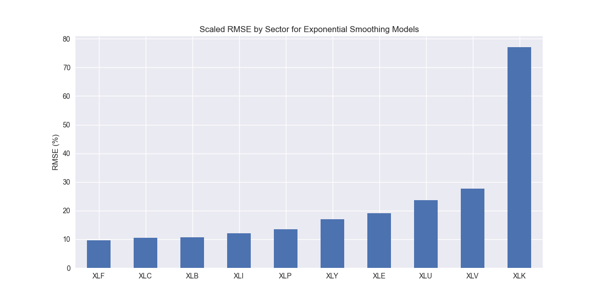
Nothing out of the ordinary. Let's compare to the benchmarks.

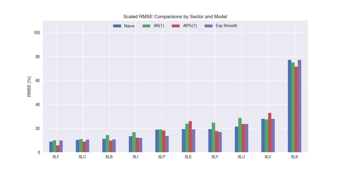
Interesting, it looks like SES might actually be better than the naïve model. It's scaled RMSE is lower than the naïve model for all but XLF, XLU, and XLC, the financial, utilities, and communications sectors. Let's confirm the aggregate performance below.

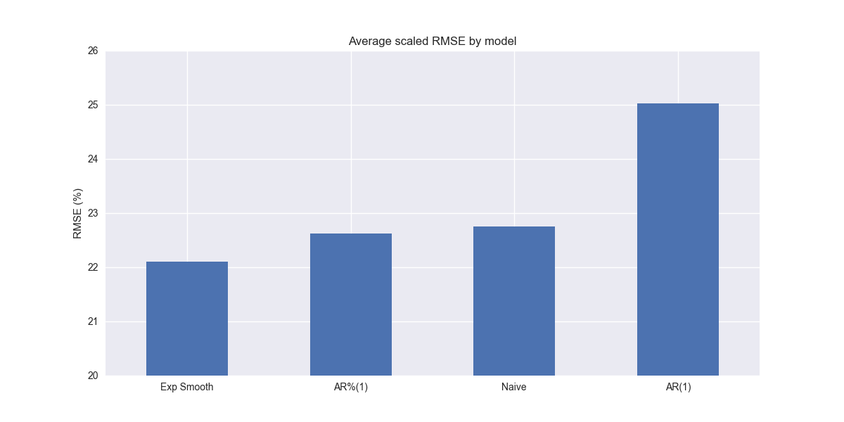
We have a new winner! Simple exponential smoothing outperforms both the naïve and autoregressive growth rate (AR%(1)) models. Of course, the differences are minimal.

Before we get too excited, recall that SES produces a flat forecast, not unlike the naïve model. That might yield the lowest overall error, but it is probably not going to win us too many friends among stakeholders that need forecasts that look realistic even if we throw in a bunch of Greek letters and derivations. We'll look at more sophisticated exponential smoothing models in our next update. Stay tuned!

Code below.

# Load packages
import numpy as np
import pandas as pd
from datetime import datetime, timedelta
import statsmodels.api as sm
import matplotlib.pyplot as plt
from matplotlib.ticker import FuncFormatter
import matplotlib as mpl
import pickle
from sktime.registry import all_estimators
from sktime.forecasting.trend import TrendForecaster

# Assign chart style
plt.style.use('seaborn-v0_8')
plt.rcParams["figure.figsize"] = (12,6)

estimators = all_estimators(
    "forecaster", as_dataframe=True, return_tags=["scitype:y", "requires-fh-in-fit"]
)

estimators.loc[estimators['scitype:y'] == 'univariate']

# Handy functions
# Functions to load and save files
def save_dict_to_file(data, filename):
    with open(filename, 'wb') as f:
        pickle.dump(data, f)

def load_dict_from_file(filename):
    with open(filename, 'rb') as f:
        return pickle.load(f)

# Create functions for indexing
def create_index(series):
    if series.iloc[0] > 0:
        return series/series.iloc[0] * 100
    else:
        return (series - series.iloc[0])/-series.iloc[0] * 100

# Function for scaled RMSE
def get_rmse_scaled(series):
    return np.sqrt(np.mean((series['actual']-series['predicted'])**2))/np.mean(series['actual'])

# Function to flatten
def flatten_df(dataf: pd.DataFrame, group_name:str, cols:list) -> pd.DataFrame:
    df_grouped = dataf.groupby(group_name)[cols].agg(list)

    for col in cols:
        df_grouped[col] = df_grouped[col].apply(lambda x: np.concatenate(x))
    
    df_long = df_grouped.apply(pd.Series.explode).reset_index()

    return df_long

# Symbols used
etf_symbols = ['XLF', 'XLI', 'XLE', 'XLK', 'XLV', 'XLY', 'XLP', 'XLB', 'XLU', 'XLC']

ticker_list = ["SHW", "LIN", "ECL", "FCX", "VMC",
               "XOM", "CVX", "COP", "WMB", "SLB",
               "JPM", "V", "MA", "BAC", "GS",
               "CAT", "RTX", "DE", "UNP", "BA",
               "AAPL", "MSFT", "NVDA", "ORCL", "CRM",
               "COST", "WMT", "PG", "KO", "PEP",
               "NEE", "D", "DUK", "VST", "SRE",
               "LLY", "UNH", "JNJ", "PFE", "MRK",
               "AMZN", "SBUX", "HD", "BKNG", "MCD",
               "META", "GOOG", "NFLX", "T", "DIS"
]

xlb = ["SHW", "LIN", "ECL", "FCX", "VMC"]
xle = ["XOM", "CVX", "COP", "WMB", "SLB"]
xlf = ["JPM", "V", "MA", "BAC", "GS"]
xli = ["CAT", "RTX", "DE", "UNP", "BA"]
xlk = ["AAPL", "MSFT", "NVDA", "ORCL", "CRM"]
xlp = ["COST", "WMT", "PG", "KO", "PEP"]
xlu = ["NEE", "D", "DUK", "VST", "SRE"]
xlv = ["LLY", "UNH", "JNJ", "PFE", "MRK"]
xly = ["AMZN", "SBUX", "HD", "BKNG", "MCD"]
xlc = ["META", "GOOG", "NFLX", "T", "DIS"]

sectors = [xlf,  xli,  xle,  xlk, xlv,  xly, xlp, xlb, xlu, xlc]

# Sector dictionary
sector_dict = {symbol.lower(): tickers for symbol, tickers in zip(etf_symbols, sectors)}
sector_map = {ticker.lower(): symbol for symbol, tickers in zip(etf_symbols, sectors) for ticker in tickers}

# Load data from disk
# See Code Walk-Throughs for how we built the data set
df_sector_dict = load_dict_from_file("path/to/data/simfin_df_rev_dict.pkl")

# Clean dataframes
df_rev_index_dict = {}
for key in sector_dict:
    temp_df = df_sector_dict[key].copy()
    col_1 = temp_df.columns[0]
    temp_df = temp_df[[col_1] + [x for x in temp_df.columns if 'revenue' in x]]
    temp_df.columns = ['date'] + [x.replace('revenue_', '').lower() for x in temp_df.columns[1:]]
    temp_idx = temp_df.copy()
    temp_idx[[x for x in temp_idx if 'date' not in x]] = temp_idx[[x for x in temp_idx if 'date' not in x]].apply(create_index)
    df_rev_index_dict[key] = temp_idx

# Create train/test dataframes
df_rev_train_dict = {}
df_rev_chg_train_dict = {}
df_rev_test_dict = {}
for key in df_rev_index_dict:
    # Create ticker list
    tickers = [x.lower() for x in sector_dict[key]]
    
    # Create dataframe fo all
    df_out = df_rev_index_dict[key]

    # Base train df
    df_train = df_out.loc[df_out['date'] < "2023-01-01"].copy()
    df_rev_train_dict[key] = df_train
    
    # Chang train df
    df_train_chg = df_train.copy()
    df_train_chg[tickers] = df_train_chg[tickers].apply(lambda x: np.log(x).diff())
    df_train_chg = df_train_chg.dropna()
    df_rev_chg_train_dict[key] = df_train_chg

    # Test df
    df_rev_test_dict[key] = df_out.loc[df_out['date'] >= "2023-01-01"]

# Create trend models
exp_models = {}
for key in df_rev_chg_train_dict:
    tickers = [x.lower() for x in sector_dict[key]]
    df_train = df_rev_train_dict[key]
    exp_models[key] = {}
    for ticker in tickers:
        try: 
            model = ExponentialSmoothing().fit(df_train[ticker])
            # model = ExponentialSmoothing(trend="add", seasonal="add", sp=4).fit(df_train[ticker])
        except ValueError as e:
            print(f"{ticker} fails due to {e}")

        exp_models[key][ticker] = model

exp_err_df = pd.DataFrame(columns = ['sector', 'ticker', 'actual', 'predicted'])
count = 0
forecast_horizon = np.arange(1,5)
for key in exp_models:
    for ticker in exp_models[key]:
        # Forecast the next 4 quarters' volatility
        y_pred = exp_models[key][ticker].predict(forecast_horizon)
        y_act = df_rev_test_dict[key][ticker].values

        exp_err_df.loc[count] = [key.upper(), ticker, y_act, y_pred]
        count += 1

for ticker in exp_err_df['ticker'].to_list():
    actual = exp_err_df.loc[exp_err_df['ticker']==ticker, 'actual'].values[0]
    predicted = exp_err_df.loc[exp_err_df['ticker']==ticker, 'predicted'].values[0]
    rmse = np.sqrt(np.mean((actual - predicted)**2))
    rmse_scaled = rmse/actual.mean()
    exp_err_df.loc[exp_err_df['ticker']==ticker, 'rmse'] = rmse
    exp_err_df.loc[exp_err_df['ticker']==ticker, 'rmse_scaled'] = rmse_scaled
  
# Clean and flatten ar_err_df
exp_df_long = flatten_df(exp_err_df, 'sector', ['actual', 'predicted'])

# Graph scaled RMSE by sector
(exp_df_long.groupby('sector')[['actual', 'predicted']].apply(get_rmse_scaled).sort_values(ascending=True)*100).plot(kind='bar', rot=0)
plt.xlabel('')
plt.ylabel('RMSE (%)')
plt.title('Scaled RMSE by Sector for Exponential Smoothing Models')
plt.show()

comp_df = pd.read_pickle("path/to/data/comp_new_df.pkl")
exp = exp_df_long.groupby('sector')[['actual', 'predicted']].apply(get_rmse_scaled).reset_index().rename(columns={0:'exp'})
comp_df = comp_df.merge(exp, how="left", on='sector')

# Plot RMSE by sector and model
(comp_df.set_index('sector')[['naive', 'lr', 'chg','exp']].sort_values('naive')*100).plot(kind='bar', rot=0)
plt.xlabel('')
plt.ylabel('RMSE (%)')
plt.ylim(0, 110)
plt.legend(['Naive', 'AR(1)', 'AR%(1)', 'Exp Smooth'], loc='upper center', ncol=4)
plt.title('Scaled RMSE Comparisons by Sector and Model')
plt.show()

# Plot Average performance
x_lab_dict = {'naive': 'Naive', 'lr': 'AR(1)', 'chg': 'AR%(1)', 'exp':'Exp Smooth'}
x_labs = comp_df.iloc[:, 1:].mean().sort_values().index.to_list()

(comp_df.iloc[:, 1:].mean().sort_values()*100).plot(kind='bar', rot=0)
plt.xticks(np.arange(4), [x_lab_dict[x] for x in x_labs])
plt.ylabel('RMSE (%)')
plt.ylim(20,26)
plt.title('Average scaled RMSE by model')
plt.show()

1. Hyndman, R.J., Athanasopoulos, G., Garza, A., Challu, C., Mergenthaler, M., & Olivares, K.G. (2024). Forecasting: Principles and Practice, the Pythonic Way. OTexts: Melbourne, Australia. Available at: OTexts.com/fpppy. Accessed on 2025-05-12.

2. The first value of the forecast is the smoothed values of the prior actuals. The second value of the forecast is the smoothed values of the first forecast value and the prior actuals. And so on. Mathematically, we say that the forecast at T + 1 is the exponential weighted average of all previous values, or y hat at T.

\(\hat{y}_{T + 1|T} = \hat{y}_{T} \)

Then the value at T + 2 is given by

\(\hat{y}_{T + 2|T + 1} = \alpha \hat{y}_{T + 1} + (1 - \alpha) \hat{y}_{T}\)

But recall that

\(\hat{y}_{T + 1} = \hat{y}_{T}\)

So we have

\(\hat{y}_{T} = \alpha \hat{y}_{T} + (1 - \alpha) \hat{y}_{T}\)

Which produces a flat forecast.