


HFW 5: Simple moving averages
Don't call them models!
In our last post, we presented an autoregressive model with four lags, AR(4). We noted that it's performance was not much different or better than the naïve and AR(1) models apart from some atrocious results in the utilities sector ETF, XLU, mainly due to Vistra (VST). We'll now look at using moving averages for forecasting.
For the present discussion, we’ll look at using a simple moving average as the basis to forecast out-of-sample values. There are, of course, more sophisticated versions—centered, weighted, and exponential moving averages, for example. But we’ll save those for another post.
Like the naïve model, the simplest forecasting method using moving averages straightlines the last value of the average over the next series of desired steps. One can also forecast recursively—as we did with the linear regression models—using prior forecast steps as inputs into the next prediction. Of course, depending on the number of forward steps that will ultimately decay to a naïve model as the last actual value becomes the only value in the average calculation.
This method does not, however, result in what is typically called a moving average model.1 When statisticians speak of moving average models, they are usually referring to something completely different. In those models, and as yet another example of statistics' love of confusing terms, the algorithms don’t actually use a moving average as we've discussed. Instead, they use past forecast errors in the following form:
It is called a moving average because the X represents a kind of weighted sum of the error terms, ‘ϵ’s, their coefficients, ‘ϕ’s, plus the intercept μ, which is often the same Greek symbol used to denote the average in a normal distribution!2 Just note that if you're using the statsmodels ARIMA class, and think you're setting the length of the moving average in the parameters, you're not. You're setting the number of lags in the error terms!
Why use a moving average? If you're a trader, moving averages should be second nature due to their widespread use in charting, technical analysis, and tactical asset allocation. Indeed, the 200-day simple moving average is probably the most prevalent and well-known example. Applying a moving average to forecasting fundamentals or some other time series follows the same logic—it smooths out the variability, revealing a more evident trend. The trick, as always, is figuring out the approximate length of the trend so you know when it's your friend...and when it's not.
Let’s now focus on performance. For this example, we’ll use three different windows—2,3, and 4 quarters—to calculate the moving average. Then, we’ll use that length of window to forecast the next values, recursively. We should note at the outset that since we only have 4 years of data—16 quarters—we’ll be losing information in an already small dataset. This constraint could diminish performance relative to benchmarks. But, so be it.
In the graph below, we show all three moving average forecasts. We call them models for sake of brevity, even though our professors will dock us points on our mid-term. Nothing in particularly jumps out at us other than in most cases the four quarter moving average tends to perform better than the two and three.

Now we show an aggregate of the moving average models vs. our benchmarks—the naïve and single lag autoregressive, AR(1), models—for each of the sectors. To aggregate the moving average models we simply average the error rates of all three. Notice how the moving average models tend to perform slightly better than the AR(1) model most of the time. The notable exceptions are at the low end of the graph.

Next, we aggregate the errors of each company, as opposed to by sector, for each model to compare overall performance. Again, not much to see here.

Finally, we find the top 10 largest errors by company for the moving average models and graph with the benchmark models.
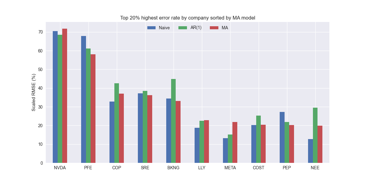
Not much that stands out, other than to show that the largest errors come from a many different sectors suggestion idiosyncratic causes..
In the end, the moving average smoothing does not perform better than the benchmarks, but doesn't perform worse. In many cases, it looks similar to the naïve model, which is no surprise given similar methodology. If we had a longer time series, we might have been able to show better performance. But we're only speculating. Now that we've tested four models—naïve, AR(1), AR(4), and moving average—evidence is emerging that no single model performs well on all companies. Additionally, all the models appear to perform poorly on those sectors with companies that exhibit explosive growth—namely, XLK with Nvidia. If this were reality, on might seek the guidance of domain expert. That person could add value to these forecasts if he or she expects, or has evidence, that the company’s trajectory will diverge from the past in a meaningful manner. Even then, forecasts still might be relatively poor. As market lore warns, inflection points in growth always surprise even the most extreme views of analysts. But that’s a story for another post. Stay tuned!
Code below
# Load packages
import pandas as pd
import numpy as np
from datetime import datetime, timedelta
import statsmodels.api as sm
from statsmodels.tsa.ar_model import AutoReg
from statsmodels.tsa.arima.model import ARIMA
import matplotlib.pyplot as plt
from matplotlib.ticker import FuncFormatter
import matplotlib as mpl
import pickle
from matplotlib.lines import Line2D
import seaborn as sns

# Assign chart style
plt.style.use('seaborn-v0_8')
plt.rcParams["figure.figsize"] = (12,6)

# Functions to load and save files
def save_dict_to_file(data, filename):
    with open(filename, 'wb') as f:
        pickle.dump(data, f)

def load_dict_from_file(filename):
    with open(filename, 'rb') as f:
        return pickle.load(f)

# Symbols used
etf_symbols = ['XLF', 'XLI', 'XLE', 'XLK', 'XLV', 'XLY', 'XLP', 'XLB', 'XLU', 'XLC']

ticker_list = ["SHW", "LIN", "ECL", "FCX", "VMC",
               "XOM", "CVX", "COP", "WMB", "SLB",
               "JPM", "V", "MA", "BAC", "GS",
               "CAT", "RTX", "DE", "UNP", "BA",
               "AAPL", "MSFT", "NVDA", "ORCL", "CRM",
               "COST", "WMT", "PG", "KO", "PEP",
               "NEE", "D", "DUK", "VST", "SRE",
               "LLY", "UNH", "JNJ", "PFE", "MRK",
               "AMZN", "SBUX", "HD", "BKNG", "MCD",
               "META", "GOOG", "NFLX", "T", "DIS"
]

xlb = ["SHW", "LIN", "ECL", "FCX", "VMC"]
xle = ["XOM", "CVX", "COP", "WMB", "SLB"]
xlf = ["JPM", "V", "MA", "BAC", "GS"]
xli = ["CAT", "RTX", "DE", "UNP", "BA"]
xlk = ["AAPL", "MSFT", "NVDA", "ORCL", "CRM"]
xlp = ["COST", "WMT", "PG", "KO", "PEP"]
xlu = ["NEE", "D", "DUK", "VST", "SRE"]
xlv = ["LLY", "UNH", "JNJ", "PFE", "MRK"]
xly = ["AMZN", "SBUX", "HD", "BKNG", "MCD"]
xlc = ["META", "GOOG", "NFLX", "T", "DIS"]

sectors = [xlf,  xli,  xle,  xlk, xlv,  xly, xlp, xlb, xlu, xlc]

# Sector dictionary
sector_dict = {symbol.lower(): tickers for symbol, tickers in zip(etf_symbols, sectors)}

# Load data from disk
# See Code Walk-Throughs for how we built the data set
df_sector_dict = load_dict_from_file("path/to/data/df_rev_dict.pkl")

# Create functions for indexing
def create_index(series):
    if series.iloc[0] > 0:
        return series/series.iloc[0] * 100
    else:
        return (series - series.iloc[0])/-series.iloc[0] * 100

# Clean dataframes
df_rev_index_dict = {}
for key in sector_dict:
    temp_df = df_sector_dict[key].copy()
    col_1 = temp_df.columns[0]
    temp_df = temp_df[[col_1] + [x for x in temp_df.columns if 'revenue' in x]]
    temp_df.columns = ['date'] + [x.replace('revenue_', '').lower() for x in temp_df.columns[1:]]
    temp_idx = temp_df.copy()
    temp_idx[[x for x in temp_idx if 'date' not in x]] = temp_idx[[x for x in temp_idx if 'date' not in x]].apply(create_index)
    df_rev_index_dict[key] = temp_idx

# Create train/test dataframes
df_rev_train_dict = {}
df_rev_test_dict = {}
for key in df_rev_index_dict:
    df_out = df_rev_index_dict[key]
    df_rev_train_dict[key] = df_out.loc[df_out['date'] < "2023-01-01"]
    df_rev_test_dict[key] = df_out.loc[df_out['date'] >= "2023-01-01"]

ma_models = {}
steps = [2,3,4]
for key in df_rev_train_dict:
    tickers = [x.lower() for x in sector_dict[key]]
    df_train = df_rev_train_dict[key]
    ma_models[key] = {}
    for ticker in tickers:
        model = pd.DataFrame(df_train[ticker]).copy()
        for step in steps:
            try:
                model[f"ma_{step}"] = model[ticker].rolling(step).mean()
            except ValueError as e:
                print(f"{ticker} fails due to {str(e)}")

        ma_models[key][ticker] = model

# Create function to forecast quarters
def forecast_next_quarters(df, ticker):
    # Dictionary to hold forecasts for each column
    forecasts = {'ticker': ticker, 'ma_2': [], 'ma_3': [], 'ma_4': []}

    # Compute forecasts for each moving average column
    for col in ['ma_2', 'ma_3', 'ma_4']:
        current_forecasts = [df[col].iloc[-1]]  # start with the last value of the moving average
        for i in range(1, 4):  # forecast the next three quarters
            # Number of actual values to include
            actuals_to_include = max(0, int(df[col].name[3]) - i)
            # Get the last few actual values from the 'Revenue' column
            actual_values = df[ticker].iloc[-actuals_to_include:].tolist()
            # Combine actual values and previous forecasts
            values_to_average = actual_values + current_forecasts[:i]
            # Compute the forecast as an average of the needed values
            new_forecast = np.mean(values_to_average)
            current_forecasts.append(new_forecast)

        # Store forecasts in the dictionary
        forecasts[col] = current_forecasts

    return pd.DataFrame(forecasts)

ma_forecasts = {}
for key in df_rev_train_dict:
    result_dfs = {ticker: forecast_next_quarters(df, ticker) for ticker, df in ma_models[key].items()}
    ma_forecasts[key] = result_dfs

# Function for scaled RMSE
def get_rmse_scaled(series, predicted):
    return np.sqrt(np.mean((series['actual']-series[predicted])**2))/np.mean(series['actual'])

err_dfs_dict = {}
for key in ma_forecasts:
    out = pd.concat(ma_forecasts[key].values(), ignore_index=True)
    out['actual'] = np.nan

    for tick in out['ticker'].unique():
        out.loc[out['ticker'] == tick, 'actual'] = df_rev_test_dict[key][tick].values

    out['sector'] = key

    err_dfs_dict[key] = out[['sector', 'ticker', 'ma_2', 'ma_3', 'ma_4', 'actual']]


ma_df = pd.concat(err_dfs_dict.values(), ignore_index=True)

# Plot moving average models
ma_plot =  (pd.concat([ma_df.groupby('sector')[['actual', ma]].apply(get_rmse_scaled, ma) for ma in ['ma_2', 'ma_3', 'ma_4']], axis=1)
            .rename(columns={0:'ma_2', 1: 'ma_3', 2:'ma_4'})
            .sort_values('ma_2', ascending=True)*100
)
ma_plot.plot(kind='bar', rot=0)
plt.xlabel('')
plt.xticks(np.arange(10), [x.upper() for x in ma_plot.index])
plt.ylabel('RMSE (%)')
plt.legend(["MA(2)", "MA(3)", "MA(4)"], loc='upper center', ncol=3)
plt.title('Scaled RMSE by Sector for MA(2-4) Models')
plt.show()


# Load comparison dataframe
comp_df = pd.read_pickle("path/to/data/comp_df.pkl")
ma = (pd.concat([ma_df.groupby('sector')[['actual', ma]].apply(get_rmse_scaled, ma) for ma in ['ma_2', 'ma_3', 'ma_4']], axis=1)
                   .mean(axis=1)).reset_index().rename(columns={0:'ma'})
ma['sector'] = [x.upper() for x in ma['sector']]
comp_df = comp_df.merge(ma, how="left", on='sector')

# Plot RMSE by sector and model
(comp_df.set_index('sector')[['naive', 'lr', 'ma']].sort_values('naive')*100).plot(kind='bar', rot=0)
plt.xlabel('')
plt.ylabel('RMSE (%)')
plt.ylim(0, 110)
plt.legend(['Naive', 'AR(1)', 'MA'], loc='upper center', ncol=3)
plt.title('Scaled RMSE Comparisons by Sector and Model')
plt.show()

# Plot RMSE by model
comp_all_df = pd.read_pickle("hello_world/data/comp_all_df.pkl")
ma_ticker = pd.concat([ma_df.groupby('ticker')[['actual', ma]].apply(get_rmse_scaled, ma) for ma in ['ma_2', 'ma_3', 'ma_4']], axis=1).mean(axis=1).reset_index().rename(columns={0:'ma'})
comp_all_df = comp_all_df.merge(ma_ticker, how="left", on='ticker')


# Violinplot
sns.violinplot(comp_all_df[['naive', 'lr', 'ma']]*100)
plt.xticks(np.arange(3), ['Naive', 'AR(1)', 'MA'])
plt.ylabel('RMSE (%)')
plt.title('Scaled RMSE by forecasting model all companies')
plt.show()

# Plot top 20% by ma
n_large = [x.upper() for x in comp_all_df.nlargest(10,"ma")['ticker'].to_list()]
(comp_all_df.nlargest(10, "ma").set_index("ticker")*100).plot(kind='bar', rot=0)
plt.xlabel('')
plt.xticks(np.arange(10), n_large)
plt.ylabel('Scaled RMSE (%)')
plt.legend(['Naive', 'AR(1)', 'MA'], loc='upper center', ncol=3)
plt.title('Top 20% highest error rate by company sorted by MA model')
plt.show()Why it isn’t called a “moving average smoothing” model, just as exponential moving average models are called “exponential smoothing” models, eludes our understanding.
In Forecasting: Principles and Practice, Rob Hyndman notes that the value of the response variable, in this case X,
“can be thought of as a weighted moving average of the past few forecast errors (although the coefficients will not normally sum to one). However, moving average models should not be confused with the moving average smoothing [discussed in Chapter 3]. A moving average model is used for forecasting future values, while moving average smoothing is used for estimating the trend-cycle of past values.”
Interesting, in Modern Time Series Forecasting, Joseph and Tackes explicitly discuss a moving average forecasting:
“A moving average forecast is another simple method that tries to overcome the pure memorization of the naïve method.”
Critically, the authors place moving averages in the section on setting baseline forecasts and further along mention ARIMA models in which “instead of past observed values, [the moving average models] use the past q errors in the forecast (which is assumed to be pure white noise) to come up with a forecast.”
Hyndman, R.J., & Athanasopoulos, G. (2021) Forecasting: principles and practice, 3rd edition, OTexts: Melbourne, Australia. OTexts.com/fpp3. Accessed on 2025-02-24.
Joseph, M. & Tackes, J, (2024) Modern Time Series Forecasting, 2nd edition, Packt Publishing: Birmingham, UK, pg 83.