HFW 7: ARMA confused

Not much different from AR or MA in aggregate

In our last post, we examined the moving average model that uses lagged error terms, not rolling averages, to forecast future revenues in our S&P 500 sector data set. While there were a few sectors that performed much better than the benchmark models—the naïve and autoregressive with one lag, AR(1)—overall performance was in line. However, we noted a trend emerging where one particular model appears to perform much better on one or two sectors than the others. We're not at a stage to examine this phenomenon in more detail, but it is something to keep in the back of our mind.

Now that we've looked at AR(1) and MA(1) models we can combine them into a, you guessed it, ARMA(1,1) model! As before, we train the model on 12 quarters of our 16 quarters of data and forecast on the remaining four. We aggregate the scaled root mean-squared error by sector and graph the results in ascending order as you see below.

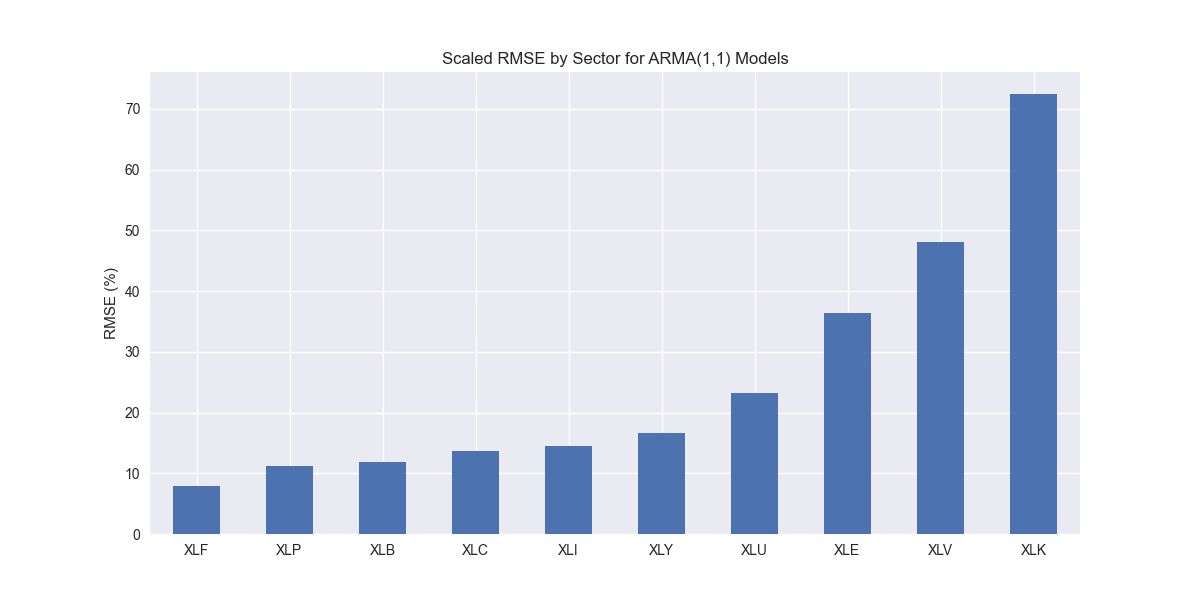
As with all the other models, XLK stands out as having the highest error. XLV and XLE are notably error prone too. We saw a similar result with the MA(1) model, so that is perhaps the cause of this trend. Additionally, while XLK remains the highest error sector, the ARMA(1,1) model produces a slightly lower result, which is positive, compared with the benchmarks. We show that below.

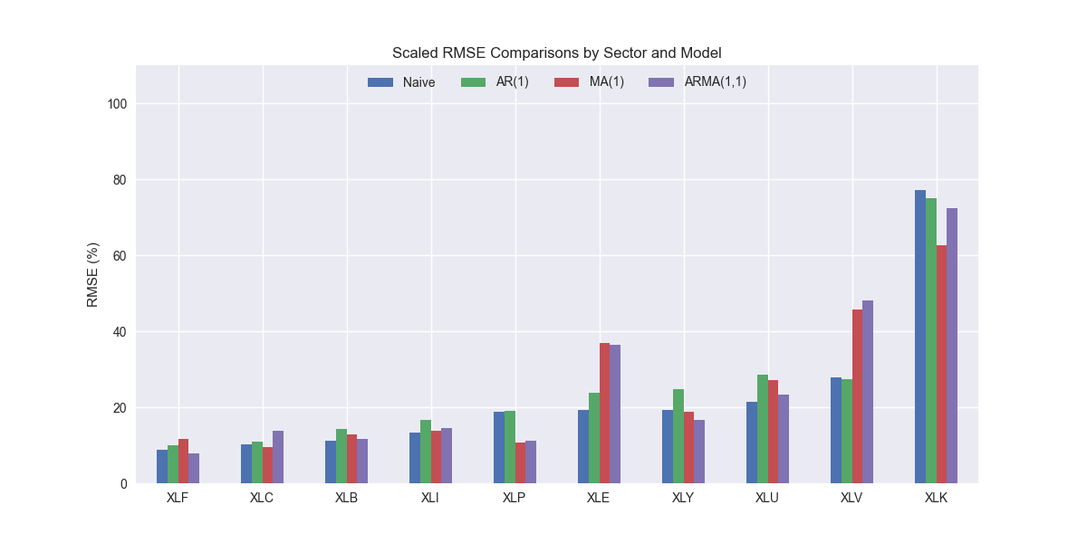
However, that the MA(1) performs better than the ARMA(1,1) model on XLK. ARMA is better on XLY and XLU, but the loss leader on XLV, though only slightly worse than MA. In aggregate, ARMA(1,1) is modestly better than MA(1), but worse than AR(1) and the naïve model. As shown in the violin plot below, it also has one or two more outliers than the MA(1) model.

This appears to come from a significantly higher error in Pfizer, ticker PFE, as shown below.

This might seem odd to folks that have followed stodgy Pfizer for a long time. But it seems to be most attributable to the ramp in revenues during the Covid-19 pandemic as shown by the XLV indexed revenue chart below.

While it is indeed strange that the ARMA(1,1) model would perform so poorly on PFE, it seems that is due to the effects of the MA(1) model, as that model performed poorly too. Have a look at the top 20% error rate chart above to confirm. Seems like the moving average model is not so good at dampening the noise as one would expect! But we mustn't be so critical. The MA model is trying to solve a problem where it has no domain knowledge by assuming that perturbations are noise. It's rather clever, but, in this case, not very useful.

Over to you. Should we test an ARMA(4,1) or ARMA(1,4) model or move on? If we do move on, you will probably have guessed which model we'll explore next—the autoregressive integrated moving average or ARIMA! Please contain your enthusiasm, but please do stay tuned!

Code below.

# Load packages
import pandas as pd
import numpy as np
from datetime import datetime, timedelta
import statsmodels.api as sm
from statsmodels.tsa.arima.model import ARIMA
from statsmodels.tsa.statespace.sarimax import SARIMAX
import matplotlib.pyplot as plt
from matplotlib.ticker import FuncFormatter
import matplotlib as mpl
import pickle
import seaborn as sns

# Assign chart style
plt.style.use('seaborn-v0_8')
plt.rcParams["figure.figsize"] = (12,6)

# Functions to load and save files
def save_dict_to_file(data, filename):
    with open(filename, 'wb') as f:
        pickle.dump(data, f)

def load_dict_from_file(filename):
    with open(filename, 'rb') as f:
        return pickle.load(f)

# Symbols used
etf_symbols = ['XLF', 'XLI', 'XLE', 'XLK', 'XLV', 'XLY', 'XLP', 'XLB', 'XLU', 'XLC']

ticker_list = ["SHW", "LIN", "ECL", "FCX", "VMC",
               "XOM", "CVX", "COP", "WMB", "SLB",
               "JPM", "V", "MA", "BAC", "GS",
               "CAT", "RTX", "DE", "UNP", "BA",
               "AAPL", "MSFT", "NVDA", "ORCL", "CRM",
               "COST", "WMT", "PG", "KO", "PEP",
               "NEE", "D", "DUK", "VST", "SRE",
               "LLY", "UNH", "JNJ", "PFE", "MRK",
               "AMZN", "SBUX", "HD", "BKNG", "MCD",
               "META", "GOOG", "NFLX", "T", "DIS"
]

xlb = ["SHW", "LIN", "ECL", "FCX", "VMC"]
xle = ["XOM", "CVX", "COP", "WMB", "SLB"]
xlf = ["JPM", "V", "MA", "BAC", "GS"]
xli = ["CAT", "RTX", "DE", "UNP", "BA"]
xlk = ["AAPL", "MSFT", "NVDA", "ORCL", "CRM"]
xlp = ["COST", "WMT", "PG", "KO", "PEP"]
xlu = ["NEE", "D", "DUK", "VST", "SRE"]
xlv = ["LLY", "UNH", "JNJ", "PFE", "MRK"]
xly = ["AMZN", "SBUX", "HD", "BKNG", "MCD"]
xlc = ["META", "GOOG", "NFLX", "T", "DIS"]

sectors = [xlf,  xli,  xle,  xlk, xlv,  xly, xlp, xlb, xlu, xlc]

# Sector dictionary
sector_dict = {symbol.lower(): tickers for symbol, tickers in zip(etf_symbols, sectors)}

# Load data from disk
# See Code Walk-Throughs for how we built the data set
df_sector_dict = load_dict_from_file("path/to/data/simfin_df_rev_dict.pkl")

# Create functions for indexing
def create_index(series):
    if series.iloc[0] > 0:
        return series/series.iloc[0] * 100
    else:
        return (series - series.iloc[0])/-series.iloc[0] * 100

# Clean dataframes
df_rev_index_dict = {}
for key in sector_dict:
    temp_df = df_sector_dict[key].copy()
    col_1 = temp_df.columns[0]
    temp_df = temp_df[[col_1] + [x for x in temp_df.columns if 'revenue' in x]]
    temp_df.columns = ['date'] + [x.replace('revenue_', '').lower() for x in temp_df.columns[1:]]
    temp_idx = temp_df.copy()
    temp_idx[[x for x in temp_idx if 'date' not in x]] = temp_idx[[x for x in temp_idx if 'date' not in x]].apply(create_index)
    df_rev_index_dict[key] = temp_idx

# Create train/test dataframes
df_rev_train_dict = {}
df_rev_test_dict = {}
for key in df_rev_index_dict:
    df_out = df_rev_index_dict[key]
    df_rev_train_dict[key] = df_out.loc[df_out['date'] < "2023-01-01"]
    df_rev_test_dict[key] = df_out.loc[df_out['date'] >= "2023-01-01"]

# Create MA model dictionary for comparison
ma_models = {}
lags = 0
diffs = 0
mas = 1
for key in df_rev_train_dict:
    tickers = [x.lower() for x in sector_dict[key]]
    df_train = df_rev_train_dict[key]
    ma_models[key] = {}
    for ticker in tickers:
        try: 
            model = ARIMA(df_train[ticker], order=(lags, diffs, mas), 
                          trend='ct',
                          enforce_stationarity=False, 
                          enforce_invertibility=False
                          ).fit()
        except ValueError as e:
            print(f"{ticker} fails due to {e}")

        ma_models[key][ticker] = model

# Function for scaled RMSE
def get_rmse_scaled(series):
    return np.sqrt(np.mean((series['actual']-series['predicted'])**2))/np.mean(series['actual'])

# Function to flatten
def flatten_df(dataf: pd.DataFrame, group_name:str, cols:list) -> pd.DataFrame:
    df_grouped = dataf.groupby(group_name)[cols].agg(list)

    for col in cols:
        df_grouped[col] = df_grouped[col].apply(lambda x: np.concatenate(x))
    
    df_long = df_grouped.apply(pd.Series.explode).reset_index()

    return df_long

# MA(1) RMSE dataframe
ma_err_df = pd.DataFrame(columns = ['sector', 'ticker', 'actual', 'predicted'])
count = 0
for key in ma_models:
    for ticker in ma_models[key]:            
        # print(f"{key}: {ticker}")
        try: 
            y_act = df_rev_test_dict[key][ticker].values
            y_pred = ma_models[key][ticker].predict(16,19, dynamic=False).values
            # y_pred = ma_models[key][ticker].forecast(4).values
        except ValueError as e:
            print(f"{ticker} fails due to {e}")
            y_act = np.nan
            y_pred = np.nan

        ma_err_df.loc[count] = [key.upper(), ticker, y_act, y_pred]
        count += 1

for ticker in ma_err_df['ticker'].to_list():
    actual = ma_err_df.loc[ma_err_df['ticker']==ticker, 'actual'].values[0]
    predicted = ma_err_df.loc[ma_err_df['ticker']==ticker, 'predicted'].values[0]
    rmse = np.sqrt(np.mean((actual - predicted)**2))
    rmse_scaled = rmse/actual.mean()
    ma_err_df.loc[ma_err_df['ticker']==ticker, 'rmse'] = rmse
    ma_err_df.loc[ma_err_df['ticker']==ticker, 'rmse_scaled'] = rmse_scaled

# Clean and flatten ar_err_df
ma_df_long = flatten_df(ma_err_df, 'sector', ['actual', 'predicted'])

# Load comparison dataframe
comp_df = pd.read_pickle("path/to/data/comp_df.pkl")
ma = ma_df_long.groupby('sector')[['actual', 'predicted']].apply(get_rmse_scaled).reset_index().rename(columns={0:'ma'})
comp_df = comp_df.merge(ma, how="left", on='sector')

# Group by tickers
ma_ticker_long = flatten_df(ma_err_df, 'ticker', ['actual', 'predicted'])
comp_all_df = pd.read_pickle("path/to/data/comp_all_df.pkl")
ma_ticker = ma_ticker_long.groupby('ticker')[['actual', 'predicted']].apply(get_rmse_scaled).reset_index().rename(columns={0:'ma'})
comp_all_df = comp_all_df.merge(ma_ticker, how="left", on='ticker')


# Built ARMA (1,1) model
# Need to use SARIMAX as it has maxiter parameter
arma_models = {}
lags = 1
diffs = 0
mas = 1
mle_retval_dict = {}
for key in df_rev_train_dict:
    tickers = [x.lower() for x in sector_dict[key]]
    df_train = df_rev_train_dict[key]
    arma_models[key] = {}
    mle_retval_dict[key] = {}
    for ticker in tickers:
        try: 
            model = SARIMAX(df_train[ticker], order=(lags, diffs, mas),
                          trend='ct', 
                          enforce_stationarity=False, 
                          enforce_invertibility=False
                          ).fit(method='powell',
                                transformed=False,
                                maxiter=100)
        except ValueError as e:
            print(f"{ticker} fails due to {e}")

        arma_models[key][ticker] = model
        if not model.mle_retvals['converged']:
            mle_retval_dict[key][ticker] = model.mle_retvals

# RMSE dataframe
arma_err_df = pd.DataFrame(columns = ['sector', 'ticker', 'actual', 'predicted'])
count = 0
for key in arma_models:
    for ticker in arma_models[key]:            
        # print(f"{key}: {ticker}")
        try: 
            y_act = df_rev_test_dict[key][ticker].values
            y_pred = arma_models[key][ticker].predict(16,19, dynamic=False).values
        except ValueError as e:
            print(f"{ticker} fails due to {e}")
            y_act = np.nan
            y_pred = np.nan

        arma_err_df.loc[count] = [key.upper(), ticker, y_act, y_pred]
        count += 1

for ticker in arma_err_df['ticker'].to_list():
    actual = arma_err_df.loc[arma_err_df['ticker']==ticker, 'actual'].values[0]
    predicted = arma_err_df.loc[arma_err_df['ticker']==ticker, 'predicted'].values[0]
    rmse = np.sqrt(np.mean((actual - predicted)**2))
    rmse_scaled = rmse/actual.mean()
    arma_err_df.loc[arma_err_df['ticker']==ticker, 'rmse'] = rmse
    arma_err_df.loc[arma_err_df['ticker']==ticker, 'rmse_scaled'] = rmse_scaled

# Clean and flatten ar_err_df
arma_df_long = flatten_df(arma_err_df, 'sector', ['actual', 'predicted'])

# Graph scaled RMSE by sector
(arma_df_long.groupby('sector')[['actual', 'predicted']].apply(get_rmse_scaled).sort_values(ascending=True)*100).plot(kind='bar', rot=0)
plt.xlabel('')
plt.ylabel('RMSE (%)')
plt.title('Scaled RMSE by Sector for ARMA(1,1) Models')
plt.show()

# Add ARMA to comparison dataframe
arma = arma_df_long.groupby('sector')[['actual', 'predicted']].apply(get_rmse_scaled).reset_index().rename(columns={0:'arma'})
comp_df = comp_df.merge(arma, how="left", on='sector')

# Plot RMSE by sector and model
(comp_df.set_index('sector')[['naive', 'lr', 'ma','arma']].sort_values('naive')*100).plot(kind='bar', rot=0)
plt.xlabel('')
plt.ylabel('RMSE (%)')
plt.ylim(0, 110)
plt.legend(['Naive', 'AR(1)', 'MA(1)', 'ARMA(1,1)'], loc='upper center', ncol=4)
plt.title('Scaled RMSE Comparisons by Sector and Model')
plt.show()

# Group by tickers
arma_ticker_long = flatten_df(arma_err_df, 'ticker', ['actual', 'predicted'])
arma_ticker = arma_ticker_long.groupby('ticker')[['actual', 'predicted']].apply(get_rmse_scaled).reset_index().rename(columns={0:'arma'})
comp_all_df = comp_all_df.merge(arma_ticker, how="left", on='ticker')

# Violinplot
sns.violinplot(comp_all_df[['naive', 'lr', 'ma', 'arma']]*100)
plt.xticks(np.arange(4), ['Naive', 'AR(1)', 'MA(1)', 'ARMA(1,1)'])
plt.ylabel('RMSE (%)')
plt.title('Scaled RMSE by forecasting model all companies')
plt.show()

# Top 20 by ARMA(1,1)
n_large = [x.upper() for x in comp_all_df.nlargest(10,"arma")['ticker'].to_list()]
(comp_all_df.nlargest(10, "arma").set_index("ticker")*100).plot(kind='bar', rot=0)
plt.xlabel('')
plt.xticks(np.arange(10), n_large)
plt.ylabel('Scaled RMSE (%)')
plt.legend(['Naive', 'AR(1)', 'MA(1)', 'ARMA(1,1)'], loc='upper center', ncol=4)
plt.title('Top 20% highest error rate by company and Model')
g")
plt.show()

# Plot XLV indexed revenues
col_names = [x.upper() for x in df_rev_index_dict['xlv'].columns[1:]] 
# df_rev_index_dict['xlv'][['date', 'pfe']].set_index('date').plot()
df_rev_index_dict['xlv'].set_index('date').plot()
plt.xlabel('')
plt.ylabel("Index")
plt.legend(col_names, loc='upper center', ncol=5)
plt.title("XLV: company indexed revenues")
plt.show()