HFW 6: Moving errors

Variable sector performance continues

In our last post, we used simple moving averages to forecast revenues for our 50 company dataset that covers the 10 of the sectors in the S&P 500. We distinguished this type of model from the one more often used in academic literature of the same name. That moving average model uses forecast errors and is called such because it represents a kind of weighted sum of the error terms, which is like a moving average. If that strikes you as convoluted or just sort of curious, then we're preaching to the choir.

As noted before, the moving average model is constructed as follows:

\(X_t = \mu + \epsilon_t + \phi_{1}\epsilon_{t-1} ++ \phi_{2}\epsilon_{t-2}+...+ \phi_{k}\epsilon_{t-k}\)

X represents a weighted sum of the error terms, ‘ϵ’s, their coefficients, ‘ϕ’s, plus the intercept μ. The assumption for this model is that the current value is some linear function of past noise and an underlying value or trend. The reason to model error terms is based on the idea that random shocks or perturbations in the data influence future values to a certain degree, but might even out over time. By modeling the white noise directly, one hopes to dampen those effects, revealing the signal at some point, like Michelangelo chipping away superfluous marble to reveal the sculpture underneath. Removing tongue from cheek…

Most fundamental analysts would probably cringe at these assumptions. Revenues, earnings, and cash flow are not random events or white noise. Shocks that occur, occur for a reason, even if the cause is not always apparent. And while one certainly wants to quantify the underlying trend, qualifying can often be teased out by channel checks and management interviews. Nonetheless, we're investigating the usefulness of the library of time series models, so we need to assess the effectiveness of moving average models.

In our first pass, we'll use a single lag in the error term, also known as as an MA(1) model. Note: in our prior post we used the abbreviation, MA(2-4), to denote moving average windows of two to four steps. We understand that this is probably confusing, but not as confusing as some of the design choices behind statsmodels.¹ Whatever the case, we show the scaled RMSE's for each sector as we've done in the past in the graph below. There are some nuances to how we built the model that are too esoteric for this discussion, but we'll touch on in our code walk-through.

It won't be evident from this stand alone graph, but the extreme error we saw in XLK in the other models, is dampened for the the MA(1) model. One can see this when we graph the MA(1) errors with the benchmark models—the naïve and autoregressive [AR(1)]—below.

Here, one can see apart from XLE and XLV, the MA(1) performs better than the benchmarks. Maybe those stats folks figured something out after all! However, looks can be somewhat deceiving, as the magnitude of error in those two ETFs more than offsets the lower errors elsewhere. The aggregate performance is pretty similar to the naïve model, but has a few outliers as show in the violin plot below.

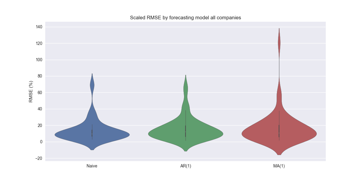
The key takeaway here is that some models continue work better for certain sectors than others. Why that is the case has yet to emerge. But it is something we are watching closely. In our next post, we'll combine an AR(1) and MA(1) model. Will it outperform the naïve model? Stay tuned!

Code below.

# Load packages
import pandas as pd
import numpy as np
from datetime import datetime, timedelta
import statsmodels.api as sm
from statsmodels.tsa.arima.model import ARIMA
import matplotlib.pyplot as plt
from matplotlib.ticker import FuncFormatter
import matplotlib as mpl
import pickle
import seaborn as sns

# Assign chart style
plt.style.use('seaborn-v0_8')
plt.rcParams["figure.figsize"] = (12,6)

# Functions to load and save files
def save_dict_to_file(data, filename):
    with open(filename, 'wb') as f:
        pickle.dump(data, f)

def load_dict_from_file(filename):
    with open(filename, 'rb') as f:
        return pickle.load(f)

# Symbols used
etf_symbols = ['XLF', 'XLI', 'XLE', 'XLK', 'XLV', 'XLY', 'XLP', 'XLB', 'XLU', 'XLC']

ticker_list = ["SHW", "LIN", "ECL", "FCX", "VMC",
               "XOM", "CVX", "COP", "WMB", "SLB",
               "JPM", "V", "MA", "BAC", "GS",
               "CAT", "RTX", "DE", "UNP", "BA",
               "AAPL", "MSFT", "NVDA", "ORCL", "CRM",
               "COST", "WMT", "PG", "KO", "PEP",
               "NEE", "D", "DUK", "VST", "SRE",
               "LLY", "UNH", "JNJ", "PFE", "MRK",
               "AMZN", "SBUX", "HD", "BKNG", "MCD",
               "META", "GOOG", "NFLX", "T", "DIS"
]

xlb = ["SHW", "LIN", "ECL", "FCX", "VMC"]
xle = ["XOM", "CVX", "COP", "WMB", "SLB"]
xlf = ["JPM", "V", "MA", "BAC", "GS"]
xli = ["CAT", "RTX", "DE", "UNP", "BA"]
xlk = ["AAPL", "MSFT", "NVDA", "ORCL", "CRM"]
xlp = ["COST", "WMT", "PG", "KO", "PEP"]
xlu = ["NEE", "D", "DUK", "VST", "SRE"]
xlv = ["LLY", "UNH", "JNJ", "PFE", "MRK"]
xly = ["AMZN", "SBUX", "HD", "BKNG", "MCD"]
xlc = ["META", "GOOG", "NFLX", "T", "DIS"]

sectors = [xlf,  xli,  xle,  xlk, xlv,  xly, xlp, xlb, xlu, xlc]

# Sector dictionary
sector_dict = {symbol.lower(): tickers for symbol, tickers in zip(etf_symbols, sectors)}

# Load data from disk
# See Code Walk-Throughs for how we built the data set
df_sector_dict = load_dict_from_file("path/to/data/df_rev_dict.pkl")

# Create functions for indexing
def create_index(series):
    if series.iloc[0] > 0:
        return series/series.iloc[0] * 100
    else:
        return (series - series.iloc[0])/-series.iloc[0] * 100

# Clean dataframes
df_rev_index_dict = {}
for key in sector_dict:
    temp_df = df_sector_dict[key].copy()
    col_1 = temp_df.columns[0]
    temp_df = temp_df[[col_1] + [x for x in temp_df.columns if 'revenue' in x]]
    temp_df.columns = ['date'] + [x.replace('revenue_', '').lower() for x in temp_df.columns[1:]]
    temp_idx = temp_df.copy()
    temp_idx[[x for x in temp_idx if 'date' not in x]] = temp_idx[[x for x in temp_idx if 'date' not in x]].apply(create_index)
    df_rev_index_dict[key] = temp_idx

# Create train/test dataframes
df_rev_train_dict = {}
df_rev_test_dict = {}
for key in df_rev_index_dict:
    df_out = df_rev_index_dict[key]
    df_rev_train_dict[key] = df_out.loc[df_out['date'] < "2023-01-01"]
    df_rev_test_dict[key] = df_out.loc[df_out['date'] >= "2023-01-01"]

# Create model dictionary
ma_models = {}
lags = 0
diffs = 0
mas = 1
for key in df_rev_train_dict:
    tickers = [x.lower() for x in sector_dict[key]]
    df_train = df_rev_train_dict[key]
    ma_models[key] = {}
    for ticker in tickers:
        try: 
            model = ARIMA(df_train[ticker], order=(lags, diffs, mas), 
                          trend='ct',
                          enforce_stationarity=False, 
                          enforce_invertibility=False
                          ).fit()
        except ValueError as e:
            print(f"{ticker} fails due to {e}")

        ma_models[key][ticker] = model

# Function for scaled RMSE
def get_rmse_scaled(series):
    return np.sqrt(np.mean((series['actual']-series['predicted'])**2))/np.mean(series['actual'])

# Function to flatten
def flatten_df(dataf: pd.DataFrame, group_name:str, cols:list) -> pd.DataFrame:
    df_grouped = dataf.groupby(group_name)[cols].agg(list)

    for col in cols:
        df_grouped[col] = df_grouped[col].apply(lambda x: np.concatenate(x))
    
    df_long = df_grouped.apply(pd.Series.explode).reset_index()

    return df_long

# RMSE dataframe
ma_err_df = pd.DataFrame(columns = ['sector', 'ticker', 'actual', 'predicted'])
count = 0
for key in ma_models:
    for ticker in ma_models[key]:            
        try: 
            y_act = df_rev_test_dict[key][ticker].values
            y_pred = ma_models[key][ticker].predict(16,19, dynamic=False).values
        except ValueError as e:
            print(f"{ticker} fails due to {e}")
            y_act = np.nan
            y_pred = np.nan

        ma_err_df.loc[count] = [key.upper(), ticker, y_act, y_pred]
        count += 1

for ticker in ma_err_df['ticker'].to_list():
    actual = ma_err_df.loc[ma_err_df['ticker']==ticker, 'actual'].values[0]
    predicted = ma_err_df.loc[ma_err_df['ticker']==ticker, 'predicted'].values[0]
    rmse = np.sqrt(np.mean((actual - predicted)**2))
    rmse_scaled = rmse/actual.mean()
    ma_err_df.loc[ma_err_df['ticker']==ticker, 'rmse'] = rmse
    ma_err_df.loc[ma_err_df['ticker']==ticker, 'rmse_scaled'] = rmse_scaled

# Clean and flatten ar_err_df
ma_df_long = flatten_df(ma_err_df, 'sector', ['actual', 'predicted'])

# Graph scaled RMSE by sector
(ma_df_long.groupby('sector')[['actual', 'predicted']].apply(get_rmse_scaled).sort_values(ascending=True)*100).plot(kind='bar', rot=0)
plt.xlabel('')
plt.ylabel('RMSE (%)')
plt.title('Scaled RMSE by Sector for MA(1) Models')
plt.show()

# Load comparison dataframe
comp_df = pd.read_pickle("path/to/data/comp_df.pkl")
ma = ma_df_long.groupby('sector')[['actual', 'predicted']].apply(get_rmse_scaled).reset_index().rename(columns={0:'ma'})
comp_df = comp_df.merge(ma, how="left", on='sector')

# Plot RMSE by sector and model
(comp_df.set_index('sector')[['naive', 'lr', 'ma']].sort_values('naive')*100).plot(kind='bar', rot=0)
plt.xlabel('')
plt.ylabel('RMSE (%)')
plt.ylim(0, 110)
plt.legend(['Naive', 'AR(1)', 'MA(1)'], loc='upper center', ncol=3)
plt.title('Scaled RMSE Comparisons by Sector and Model')
plt.show()

# Group by tickers
arma_ticker_long = flatten_df(ma_err_df, 'ticker', ['actual', 'predicted'])

comp_all_df = pd.read_pickle("path/to/data/comp_all_df.pkl")
ma_ticker = arma_ticker_long.groupby('ticker')[['actual', 'predicted']].apply(get_rmse_scaled).reset_index().rename(columns={0:'ma'})
comp_all_df = comp_all_df.merge(ma_ticker, how="left", on='ticker')

# Violinplot
sns.violinplot(comp_all_df[['naive', 'lr', 'ma']]*100)
plt.xticks(np.arange(3), ['Naive', 'AR(1)', 'MA(1)'])
plt.ylabel('RMSE (%)')
plt.title('Scaled RMSE by forecasting model all companies')
plt.show()

1. It is not at all clear to us why statsmodels forces one to use a more advanced class like SARIMAX simply to be able to set the max iteration parameter for an ARIMA model! In our code walk-through we'll build some of these models from scratch, which should make some our choices more explicit.