Outperforming with momentum

The premier anomaly

Just a quick note today as we’ve finished up most of the code walk-throughs to build the revenue dataset for the Hello Forecasting World [HFW] series. We've discussed momentum in the past, particularly in our #30daysofbacktesting series, where we used it to forecast forward returns which in turn generated trading signals. As Nobel Prize winner Eugene Fama has said, "The premier anomaly is momentum." And certainly for us, momentum remains one of the most interesting artifacts of quantitative investing. Today, we want to look at whether we can use momentum to outperform the S&P 500. And since we've already been using the SPDRS—that is, the ETFs that track the performance of the 10 or so sectors in the S&P—we figured we’d use those assets to do it!

Here's the set up. We'll use a lookback period of around 120 trading days, or roughly a half year to calculate momentum. The calculation will simply be the the price return at the end of the period vs the beginning for each of the ETFs. We then rank those returns cross-sectionally. We’ll go long the top five and short the bottom one ETF. The longs are equally-weighted between them, while the short is only 20% of the total portfolio value. The momentum portfolio is rebalanced monthly. The cumulative return profile, looks like the following.

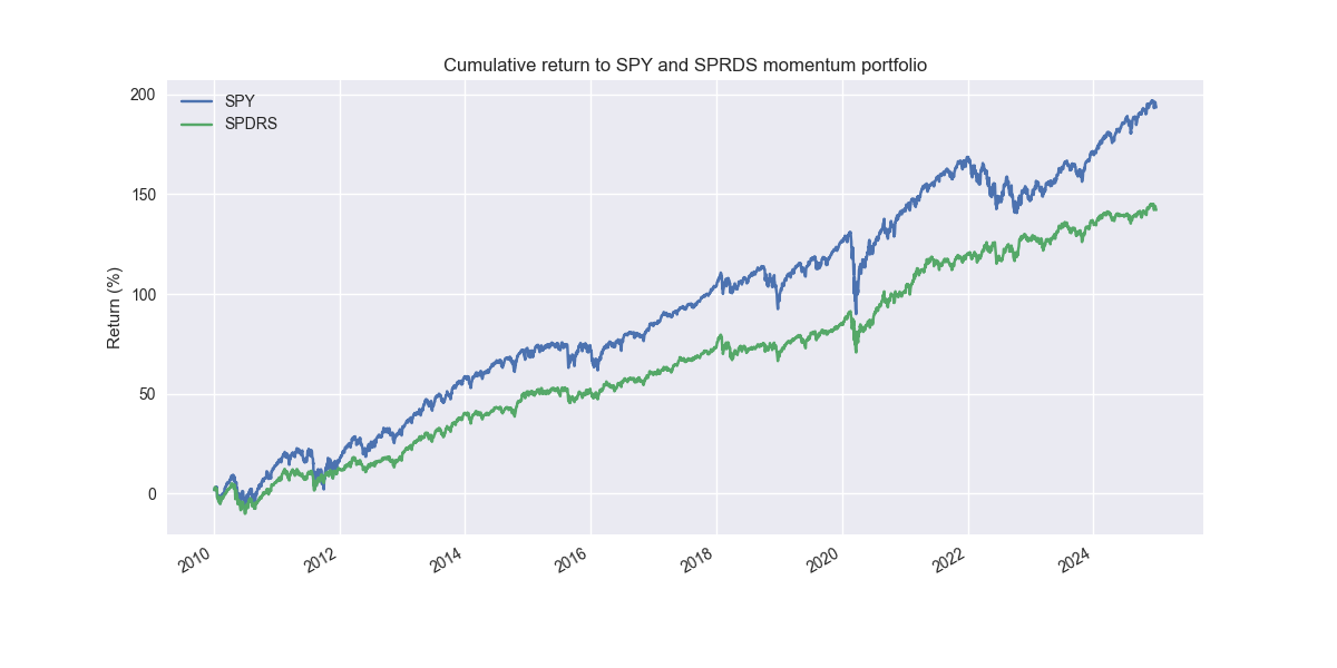
Now we admit that this graph is not that exciting. The momentum portfolio underperforms. But note how smooth the return curve is compared to the S&P. Many folks would find such a curve quite attractive. Indeed, the Sharpe ratio for the momentum strategy is about 4pts higher at 0.80 vs. 0.76 for the S&P. The main reason for this, despite significantly lower returns, is the momentum portfolio’s volatility is roughly 70% of the S&P. Hence, if added a small amount of leverage, rescaling the returns by the ratio of the S&P to the momentum volatility, we'd get the following performance graph.

In this case, the Sharpe Ratio remains the same, but cumulative returns increase by 10ppts! Not bad. But one will notice that most of the performance comes from avoiding the interest rate wreck in the 2022-2023 period. That should make the hair on the back your head stand up because we don’t know when such a market will repeat itself. That said, the momentum portfolio did not suffer as severe a drawdown in 2022 as the SPY.

Of course, there’s definitely some snooping going on here. So if really wanted to test this rigorously, we needed to set up some nice train/test splits as well as perform a grid search on the parameters we chose. But we’ll save that for another post. Until then, stay tuned!

Code below

# Load libraries
import pandas as pd
import numpy as np
import yfinance as yf
from datetime import datetime, timedelta
import matplotlib.pyplot as plt

# Plotting parameters
plt.style.use("seaborn-v0_8")
plt.rcParams['figure.figsize'] = (12,6)

# Symbols used
symbols = ['XLF', 'XLI', 'XLE', 'XLK', 'XLV', 'XLY', 'XLP', 'XLB', 'XLU', 'XLC']

# Functions
def get_momentum_rank(price_data, steps):

    pad_arr = np.zeros((steps, price_data.shape[1]))
    sig_arr = price_data.iloc[steps:].values/price_data.iloc[:-steps].values - 1
    tot_arr = np.vstack((pad_arr, sig_arr))
    momo = pd.DataFrame(tot_arr, columns=price_data.columns, index=price_data.index)
    return momo.rank(axis=1)

def mark_highest_lowest(dataf, longs=2, shorts=2, short=True):
    markers = np.zeros(dataf.shape, dtype=int)  # Initialize with zeros

    # Get column positions of 2 highest and 2 lowest values for each row
    highest_idx = np.argsort(-dataf.values, axis=1)[:, :longs]  # Negative sign to get largest
    if short:
        lowest_idx = np.argsort(dataf.values, axis=1)[:, :shorts]  # Smallest values directly

    # Use advanced indexing to assign values
    row_idx = np.arange(dataf.shape[0])[:, None]  # Row indices to align with column indices
    markers[row_idx, highest_idx] = 1  # Assign 1 to highest
    if short:
        markers[row_idx, lowest_idx] = -1  # Assign -1 to lowest

    # Convert back to DataFrame
    return pd.DataFrame(markers, index=dataf.index, columns=dataf.columns)

def calculate_portfolio_returns(returns, signals, longs=5, shorts=1, rebalance=False, frequency='month', long_weight=1.0, short_weight=0.2):

    # Ensure returns and signals line up
    returns = returns.copy()
    signals = signals.reindex(returns.index).fillna(0)
    
    # Create a frequency-based set of rebalancing dates if rebalance=True
    if rebalance:
        if frequency == 'week':
            rebal_dates = returns.resample('W-FRI').last().index
        elif frequency == 'month':
            rebal_dates = returns.resample('ME').last().index
        elif frequency == 'quarter':
            rebal_dates = returns.resample('QE').last().index
        else:
            # default to daily if frequency is unrecognized
            rebal_dates = returns.index
    else:
        rebal_dates = pd.DatetimeIndex([])  # no scheduled rebal dates

    # Initialize day 0 weights to zero (no positions)
    weight_prev = pd.Series(0.0, index=returns.columns)
    
    # Lists to store the output
    daily_returns_list = []
    weight_list = []
    
    # Iterate over each date
    all_dates = returns.index
    for i, dt in enumerate(all_dates):
        if i == 0:
            # We record daily return = 0.0, keep weights = 0.0 on day 1
            daily_returns_list.append(0.0)
            weight_list.append(weight_prev.values)
            continue
        
        # Calculate the portfolio's daily return based on yesterday's weights
        daily_ret = returns.iloc[i]
        port_r = (weight_prev * daily_ret).sum()  )
        
        #"Drift" the weights by multiplying by returns
        new_weights = weight_prev * (1.0 + daily_ret)
        sum_w = new_weights.abs().sum()
        if sum_w > 0:
            # normalize so total absolute weights sum to 1
            new_weights /= sum_w  
        else:
            # If everything was zero or no active positions, remain zero
            new_weights = weight_prev.copy()
        
        # Check if signals changed or if it's a scheduled rebal date
        sig_yesterday = signals.iloc[i-1]
        sig_today = signals.iloc[i]
        changed = not sig_yesterday.equals(sig_today)
        scheduled_rebal = dt in rebal_dates
        
        if changed or scheduled_rebal:
            # Recompute fresh weights from today's signals
            longs_idx = sig_today[sig_today == 1].index
            shorts_idx = sig_today[sig_today == -1].index
            
            n_longs = len(longs_idx)
            n_shorts = len(shorts_idx)
            
            w_fresh = pd.Series(0.0, index=returns.columns)
            if n_longs > 0:
                w_fresh[longs_idx] = long_weight / n_longs
            if n_shorts > 0:
                w_fresh[shorts_idx] = -(short_weight / n_shorts)
            
            new_weights = w_fresh
        
        # Store the result
        daily_returns_list.append(port_r)
        weight_list.append(new_weights.values)
        
        # Update for next iteration
        weight_prev = new_weights
    
    # Build final objects
    daily_portfolio_returns = pd.Series(daily_returns_list, index=all_dates, name='SPDRS')
    weight_history = pd.DataFrame(weight_list, index=all_dates, columns=returns.columns)
    
    return daily_portfolio_returns, weight_history

# Data
spy = yf.download("SPY", start='2000-01-01', end='2025-01-01')
spy_price = spy['Close']
spy_ret = spy_price.apply(lambda x: np.log(x/x.shift()))

data = yf.download(symbols, start='2000-01-01', end='2025-01-01')
price = data['Close']
returns = price.apply(lambda x: np.log(x/x.shift()))

# Calculate returns
ret_rank = get_momentum_rank(price, 120)
ret_sig = mark_highest_lowest(ret_rank, longs=5, shorts=1, short=True)
ret_pnl = returns * ret_sig.shift()

# Calculate returns and merge with SPY
strat_df, _ = calculate_portfolio_returns(returns, ret_sig.shift(1), longs=5, shorts=1, rebalance=True, frequency='month', long_weight=1.0, short_weight=0.2)
perf_df = pd.concat([spy_ret, strat_df], axis=1)

# Plot performance
(perf_df.loc["2010":].cumsum()*100).plot()
plt.xlabel("")
plt.ylabel('Return (%)')
plt.legend(['SPY', 'SPDRS'])
plt.title("Cumulative return to SPY and SPRDS momentum portfolio")
plt.show()

# Equalize volatility
vol_1 = perf_df.loc["2010":, 'SPY'].std()*np.sqrt(252)
vol_2 = perf_df.loc["2010":, 'SPDRS'].std()*np.sqrt(252)
scaled_returns = perf_df.loc["2010":, 'SPDRS']*(vol_1 / vol_2)

# Merge scaled returns with SPY
perf_2_df = pd.concat([spy_ret.loc["2010":], scaled_returns], axis=1)

# Plot performance
(perf_2_df.cumsum()*100).plot()
plt.xlabel("")
plt.ylabel('Return (%)')
plt.legend(['SPY', 'SPDRS'])
plt.title("Cumulative return to SPY and levered SPRDS momentum portfolio")
plt.show()