


HFW 19: Automate ETS
AutoETS improves forecasts meaningfully vs. ETS on Apple
In our last post, we introduced the ETS model, which is an exponential smoothing model for Trend and Seasonality that includes an Error term, hence ETS. Why it isn't called TSE, rather than ETS since the error innovation only came later, is anyone's guess. Whatever the case, employing this model saw a modest improvement in performance relative to the naive and autoregressive growth (AR1(%)) benchmarks. It also outperformed the simple exponential smoothing (SES) model, though the differences were minor.
Having set up the ETS model, we can now introduce AutoETS, which is simply an automated way to select the best parameters from the nine different combinations of error, trend, and seasonality that are either additive or multiplication. We were remiss to mention in our prior post that the ETS model was originally developed in couple of key papers from 1997 and 20021 and covered in detail in a book by the great Rob Hyndman and others: Forecasting with Exponential Smoothing: The State Space Approach. Recall, ETS models are referred to as innovations state space models where "state space" comes from multiple equations: one that describes the observed data and the others that describe how the other components—level, trend, or seasonality, in other words, states—change over time. The "innovations" part is that all equations use the same random error process.
That's enough history. Time for us to stand on the shoulders of giants. Before we do, we should first explain some terminology. When folks discuss a particular ETS model you might see something like ETS(NAM). The letters inside the parentheses stand for None, Additive, and Multiplicative aligning with Error, Trend, and Seasonality. Hence, the model we showed in our last post was an ETS(AAA) model, as each of the states was assumed to be additive (More on additive vs. multiplicative in a later post). AutoETS finds the best configuration of those nine possible combinations of ETS and NAM.
Before we deploy AutoETS on our data set in the next post, we’ll look at single example where we compare an ETS(AAA) model from our last post to an AutoETS model on Apple. Let's go!
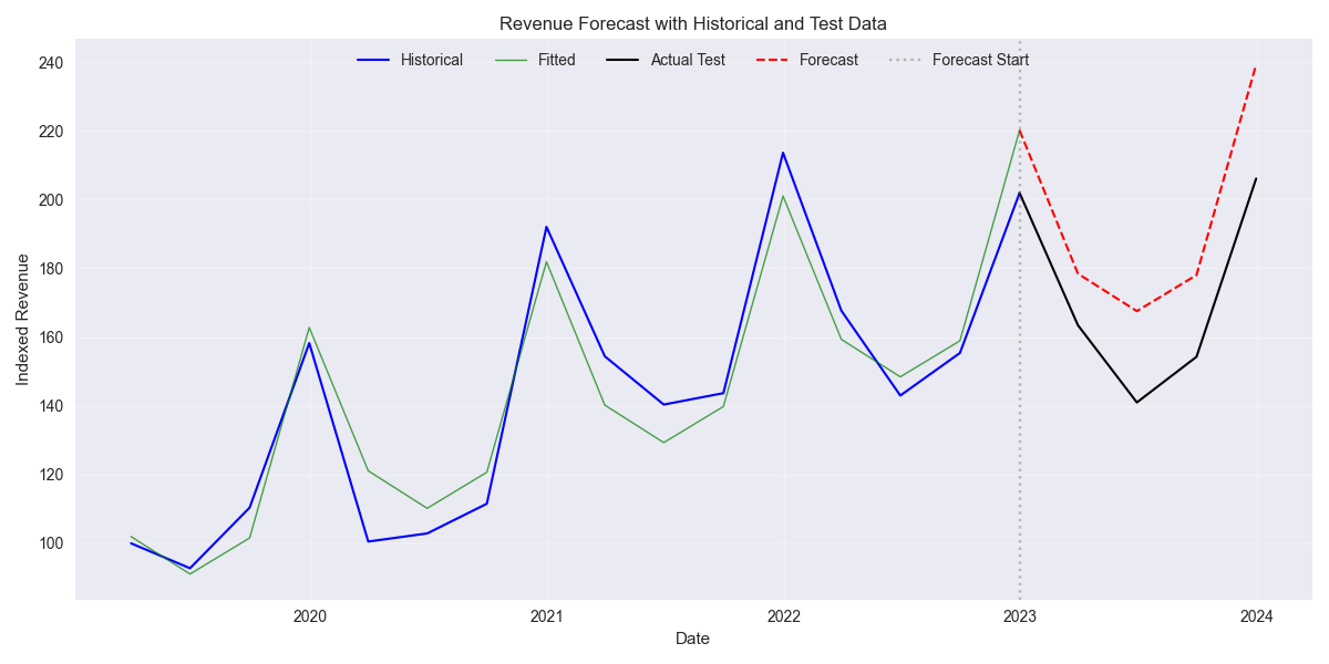
In the first graph, we show the ETS(AAA) model with the fitted values on the training set and the forecast values. As one can see, the fitted values follow the shape of Apple's revenues nicely. The forecast looks pretty good too. Recall, one of the reasons one might favor an SES or ETS model over a naive one, even if the naive's error rate is lower, is that the forecasts actually look like forecasts. In any case, the root mean-squared error (RMSE) for the ETS(AAA) model is about 25 (which doesn’t really tell you much) and the scaled RSMSE is 15%. In other words, the RMSE of the forecasts is a fraction of average actuals. That's pretty good given that the aggregate scaled RMSE for XLK has tracked the 70-80% range out of all the different models we've tried. Of course, that is mainly due to the inclusion of Nvidia.
Let's see what AutoETS can do. We only show the forecasts for ETS(AAA) and AutoETS below.

Clearly, AutoETS follows the actual revenues in the test much more closely. Critically, the scaled RMSE for the AutoETS model is only about 5%, a 66% reduction in error! (Don't you love when you can use the change in percentages to make a dramatic point!) Plus one for the AutoETS model. Of course, this is only one instance. But we are curious to find out what AutoETS decided were the best parameters. It turns out it was an MNA model, or, in other words Multiplicative Errors, No Trend, and Additive Seasonality.
We'll look at this in more detail as well as the mechanics of putting the Auto in AutoETS. But for now this is an encouraging development and we're looking forward to seeing how AutoETS performs on the full dataset. Stay tuned!
Code below.
# Load packages
import numpy as np
import pandas as pd
from datetime import datetime, timedelta
import statsmodels.api as sm
import matplotlib.pyplot as plt
from matplotlib.ticker import FuncFormatter
import matplotlib as mpl
import pickle
from statsmodels.tsa.exponential_smoothing.ets import ETSModel
from sktime.forecasting.ets import AutoETS

# Assign chart style
plt.style.use('seaborn-v0_8')
plt.rcParams["figure.figsize"] = (12,6)

# Handy functions
# Functions to load and save files
def save_dict_to_file(data, filename):
    with open(filename, 'wb') as f:
        pickle.dump(data, f)

def load_dict_from_file(filename):
    with open(filename, 'rb') as f:
        return pickle.load(f)

# Create functions for indexing
def create_index(series):
    if series.iloc[0] > 0:
        return series/series.iloc[0] * 100
    else:
        return (series - series.iloc[0])/-series.iloc[0] * 100

# Function for scaled RMSE
def get_rmse_scaled(series):
    return np.sqrt(np.mean((series['actual']-series['predicted'])**2))/np.mean(series['actual'])

# Function to flatten
def flatten_df(dataf: pd.DataFrame, group_name:str, cols:list) -> pd.DataFrame:
    df_grouped = dataf.groupby(group_name)[cols].agg(list)

    for col in cols:
        df_grouped[col] = df_grouped[col].apply(lambda x: np.concatenate(x))

    df_long = df_grouped.apply(pd.Series.explode).reset_index()

    return df_long

# Symbols used
etf_symbols = ['XLF', 'XLI', 'XLE', 'XLK', 'XLV', 'XLY', 'XLP', 'XLB', 'XLU', 'XLC']

ticker_list = ["SHW", "LIN", "ECL", "FCX", "VMC",
               "XOM", "CVX", "COP", "WMB", "SLB",
               "JPM", "V", "MA", "BAC", "GS",
               "CAT", "RTX", "DE", "UNP", "BA",
               "AAPL", "MSFT", "NVDA", "ORCL", "CRM",
               "COST", "WMT", "PG", "KO", "PEP",
               "NEE", "D", "DUK", "VST", "SRE",
               "LLY", "UNH", "JNJ", "PFE", "MRK",
               "AMZN", "SBUX", "HD", "BKNG", "MCD",
               "META", "GOOG", "NFLX", "T", "DIS"
]

xlb = ["SHW", "LIN", "ECL", "FCX", "VMC"]
xle = ["XOM", "CVX", "COP", "WMB", "SLB"]
xlf = ["JPM", "V", "MA", "BAC", "GS"]
xli = ["CAT", "RTX", "DE", "UNP", "BA"]
xlk = ["AAPL", "MSFT", "NVDA", "ORCL", "CRM"]
xlp = ["COST", "WMT", "PG", "KO", "PEP"]
xlu = ["NEE", "D", "DUK", "VST", "SRE"]
xlv = ["LLY", "UNH", "JNJ", "PFE", "MRK"]
xly = ["AMZN", "SBUX", "HD", "BKNG", "MCD"]
xlc = ["META", "GOOG", "NFLX", "T", "DIS"]

sectors = [xlf,  xli,  xle,  xlk, xlv,  xly, xlp, xlb, xlu, xlc]

# Sector dictionary
sector_dict = {symbol.lower(): tickers for symbol, tickers in zip(etf_symbols, sectors)}
sector_map = {ticker.lower(): symbol for symbol, tickers in zip(etf_symbols, sectors) for ticker in tickers}

# Load data from disk
# See Code Walk-Throughs for how we built the data set
df_sector_dict = load_dict_from_file("path/to/data/simfin_df_rev_dict.pkl")

# Clean dataframes
df_rev_index_dict = {}
for key in sector_dict:
    temp_df = df_sector_dict[key].copy()
    col_1 = temp_df.columns[0]
    temp_df = temp_df[[col_1] + [x for x in temp_df.columns if 'revenue' in x]]
    temp_df.columns = ['date'] + [x.replace('revenue_', '').lower() for x in temp_df.columns[1:]]
    temp_idx = temp_df.copy()
    temp_idx[[x for x in temp_idx if 'date' not in x]] = temp_idx[[x for x in temp_idx if 'date' not in x]].apply(create_index)
    df_rev_index_dict[key] = temp_idx

# Create train/test dataframes
df_rev_train_dict = {}
df_rev_chg_train_dict = {}
df_rev_test_dict = {}
for key in df_rev_index_dict:
    # Create ticker list
    tickers = [x.lower() for x in sector_dict[key]]

    # Create dataframe fo all
    df_out = df_rev_index_dict[key]

    # Base train df
    df_train = df_out.loc[df_out['date'] < "2023-01-01"].copy()
    df_rev_train_dict[key] = df_train

    # Chang train df
    df_train_chg = df_train.copy()
    df_train_chg[tickers] = df_train_chg[tickers].apply(lambda x: np.log(x).diff())
    df_train_chg = df_train_chg.dropna()
    df_rev_chg_train_dict[key] = df_train_chg

    # Test df
    df_rev_test_dict[key] = df_out.loc[df_out['date'] >= "2023-01-01"]

# Forecast comparison
y = df_rev_train_dict['xlk']['aapl']
y_act = df_rev_test_dict['xlk']['aapl']

hist_dates = df_rev_train_dict['xlk']['date']
forecast_dates = df_rev_test_dict['xlk']['date']

# Fit ETS model: Error='add', Trend='add', Seasonality='add'
ets = ETSModel(
    y,
    error='add',          # 'add' or 'mul'
    trend='add',          # 'add', 'mul', or None
    seasonal='add',       # 'add', 'mul', or None
    seasonal_periods=4
)
fit = ets.fit(disp=False)

forecast = fit.get_prediction(start=16, end=19)

# # Get the last value of y to connect predictions and actual
last_y_value = y.iloc[-1]
last_y_date = hist_dates.iloc[-1]

# Plot
plt.figure()

# Plot historical data
plt.plot(hist_dates, y, 'b-', label='Historical', linewidth=1.5)

# Plot fitted values
plt.plot(hist_dates, fit.fittedvalues, 'g-', label='Fitted', linewidth=1, alpha=0.7)

# Plot actual test values connecting to last historical value
plt.plot([last_y_date] + list(forecast_dates),
         [last_y_value] + list(y_act.values),
         'k-', label='Actual Test', linewidth=1.5)

# Plot forecast values connecting to last fitted value
last_fitted_value = fit.fittedvalues.iloc[-1]
plt.plot([last_y_date] + list(forecast_dates),
         [last_fitted_value] + list(forecast.predicted_mean),
         'r--', label='Forecast', linewidth=1.5)

# Add vertical line to separate historical and forecast periods
plt.axvline(x=last_y_date, color='gray', linestyle=':', alpha=0.5, label='Forecast Start')

plt.title('Revenue Forecast with Historical and Test Data')
plt.xlabel('Date')
plt.ylabel('Indexed Revenue')
plt.legend(loc='upper center', ncol=5)
plt.grid(True, alpha=0.3)
plt.tight_layout()
plt.show()

# Get error
ets_rmse = np.sqrt(np.mean((y_act - forecast.predicted_mean)**2))
ets_rmse_scaled = ets_rmse/y_act.mean()

# Auto ETS
fh = np.arange(1,5)
auto_ets = AutoETS(
    auto=True,
    n_jobs=-1,          # 'add' or 'mul'
    sp=4
)
auto_ets.fit(y)

y_pred = auto_ets.predict(fh=fh)

# Plot
plt.figure()

# Plot y with historical dates
plt.plot(hist_dates, y.values, 'b-', label='Historical', linewidth=1.5)

# Get the last value of y to connect predictions and actual
last_y_value = y.iloc[-1]
last_y_date = hist_dates.iloc[-1]

# Plot y_act connecting to last y value
plt.plot([last_y_date] + list(forecast_dates),
         [last_y_value] + list(y_act.values),
         'g-', label='Actual', linewidth=1.5)

# Plot predictions with dashed lines, starting from the last y value
plt.plot([last_y_date] + list(forecast_dates),
         [last_y_value] + list(forecast.predicted_mean),
         'r--', label='ETS Forecast', linewidth=1)

plt.plot([last_y_date] + list(forecast_dates),
         [last_y_value] + list(y_pred.values),
         color='purple', linestyle='--', label='AutoETS Forecast', linewidth=1)

plt.axvline(x=last_y_date, color='gray', linestyle=':', alpha=0.5, label='Forecast Start')
plt.legend(loc='upper center', ncol=5)
plt.title('ETS and AutoETS Revenue Forecasts Comparison for AAPL')
plt.xlabel('')
plt.ylabel('Indexed Revenue')
plt.show()

# Get error
autoets_rmse = np.sqrt(np.mean((y_act - y_pred)**2))
autoets_rmse_scaled = autoets_rmse/y_act.mean()