


HFW 2: OLS Workhorse
We use the workhorse linear regression model to forecast four quarters of revenues for each of the five companies we selected from the ten S&P sectors
On our last post, we outlined the basic dataset we plan to use for this series and summarized how we built it. For further details on the process, please check out Code Walk-Throughs. We then established our benchmark, a naïve forecast that straightlines the last value for the next four quarters in our test set. Nothing really stood out from the graph of the scaled root mean-squared error (RMSE) that we presented other than outsized error of around 75% in XLK, mainly due to Nvidia's outsized growth in 2023.
Now that we've established a baseline, we'll discuss our first model—the workhorse, the ubiquitous linear regression. Our intention is to use univariate models throughout this series. That is, as we define it, only a single independent variable will forecast the dependent variable.1 That independent variable may be twisted, tortured, and differenced into multiple other features, but the key point is that we won't be adding exogenous variables to these models.2 The independent variable will simply be a lagged version of the dependent. Hence, properly stated, this first model is autoregressive, but let's not worry too much about that right now. This process will become clear when we look at more sophisticated models.
We need to take a quick detour to discuss the modeling strategy. If you have 1,...,k instances of variable x and you want to forecast the k + 1 instance using the kth, then you'd set up the univariate equation such that for
In our case, we want to forecast k + [1, 2, 3, 4] , or the next four instances in the sequence, equivalent to the next four quarters. Normally, that might be done by rolling forward the model. But we can't do that, because we're assuming that, like our junior analyst, we're sitting in front of our (Oh horror!) Excel model after the fourth quarter conference call trying to figure out what we're going to forecast for the next four quarters. It would be so nice to automate this. But, since we don't know Python or R, we're stuck using a thumb in the wind and CTRL + R for the last 4 quarter growth rates and then we get a call from a client asking what we’re assuming for next quarter and we haven’t even published the model yet and... We digress.
The question is, how do we forecast out four quarters using a single period lag if we don't have the actual values to forecast? We have 20 quarters of data, of which 16 are used to train the model and the remaining four are used as out-of-sample tests. The model needs a prior value as an input to make a forecast. For quarter 17, it has the actual value of quarter 16 from the training set. But for quarters 18, 19, and 20, it has nothing. Many time series packages will use the model to make recursive forecasts from prior forecasts. That is, the forecast for quarter 16 is used as input to forecast quarter 17, and the forecast for quarter 17 as input to forecast quarter 18, and so on. Clearly, using a forecast as an actual will tend to magnify errors as one forecasts further out in time. But that is a discussion for another post.
We’ll use that same methodology to build the forecasts using a single period lag and aggregate the results by sector. We graph the scaled RMSE below.
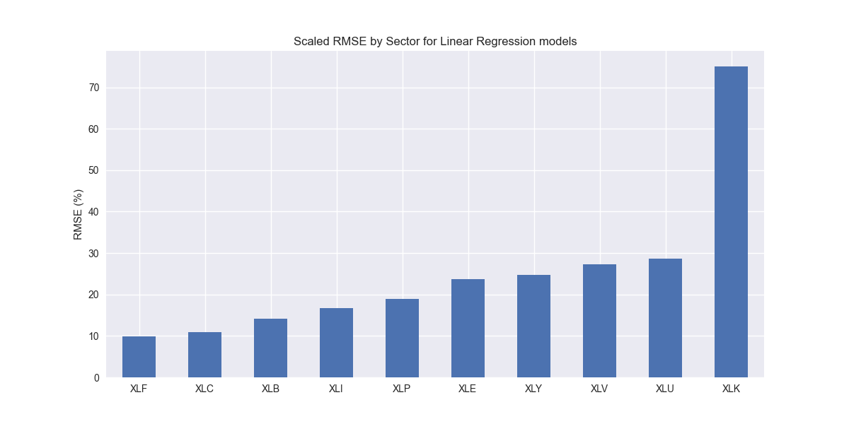
The results don't look too different from the naïve forecast, with XLK showing the most dramatic error. We'll discuss these results in more detail when we compare the two models in our next post. Stay tuned.
Code below
# Load packages
import pandas as pd
import numpy as np
from datetime import datetime, timedelta
import statsmodels.api as sm
import matplotlib.pyplot as plt
from matplotlib.ticker import FuncFormatter
import matplotlib as mpl
import pickle

# Assign chart style
plt.style.use('seaborn-v0_8')
plt.rcParams["figure.figsize"] = (12,6)

# Functions to load files
# Load and save
def save_dict_to_file(data, filename):
    with open(filename, 'wb') as f:
        pickle.dump(data, f)

def load_dict_from_file(filename):
    with open(filename, 'rb') as f:
        return pickle.load(f)

# Symbols used
etf_symbols = ['XLF', 'XLI', 'XLE', 'XLK', 'XLV', 'XLY', 'XLP', 'XLB', 'XLU', 'XLC']

ticker_list = ["SHW", "LIN", "ECL", "FCX", "VMC",
               "XOM", "CVX", "COP", "WMB", "SLB",
               "JPM", "V", "MA", "BAC", "GS",
               "CAT", "RTX", "DE", "UNP", "BA",
               "AAPL", "MSFT", "NVDA", "ORCL", "CRM",
               "COST", "WMT", "PG", "KO", "PEP",
               "NEE", "D", "DUK", "VST", "SRE",
               "LLY", "UNH", "JNJ", "PFE", "MRK",
               "AMZN", "SBUX", "HD", "BKNG", "MCD",
               "META", "GOOG", "NFLX", "T", "DIS"
]

xlb = ["SHW", "LIN", "ECL", "FCX", "VMC"]
xle = ["XOM", "CVX", "COP", "WMB", "SLB"]
xlf = ["JPM", "V", "MA", "BAC", "GS"]
xli = ["CAT", "RTX", "DE", "UNP", "BA"]
xlk = ["AAPL", "MSFT", "NVDA", "ORCL", "CRM"]
xlp = ["COST", "WMT", "PG", "KO", "PEP"]
xlu = ["NEE", "D", "DUK", "VST", "SRE"]
xlv = ["LLY", "UNH", "JNJ", "PFE", "MRK"]
xly = ["AMZN", "SBUX", "HD", "BKNG", "MCD"]
xlc = ["META", "GOOG", "NFLX", "T", "DIS"]

sectors = [xlf,  xli,  xle,  xlk, xlv,  xly, xlp, xlb, xlu, xlc]

# Sector dictionary
sector_dict = {symbol.lower(): tickers for symbol, tickers in zip(etf_symbols, sectors)}

# Load data from disk
# See Code Walk-Throughs for how we built the data set
df_sector_dict = load_dict_from_file("path/to/df_rev_dict.pkl")

# Create functions for indexing
def create_index(series):
    if series.iloc[0] > 0:
        return series/series.iloc[0] * 100
    else:
        return (series - series.iloc[0])/-series.iloc[0] * 100

# Clean dataframes
df_rev_index_dict = {}
for key in sector_dict:
    temp_df = df_sector_dict[key].copy()
    col_1 = temp_df.columns[0]
    temp_df = temp_df[[col_1] + [x for x in temp_df.columns if 'revenue' in x]]
    temp_df.columns = ['date'] + [x.replace('revenue_', '').lower() for x in temp_df.columns[1:]]
    temp_idx = temp_df.copy()
    temp_idx[[x for x in temp_idx if 'date' not in x]] = temp_idx[[x for x in temp_idx if 'date' not in x]].apply(create_index)
    df_rev_index_dict[key] = temp_idx

# Print dataframes for quick spot checking
for key in sector_dict:
    print(key)
    print(df_rev_index_dict[key].head())
    print('')

# Create train/test dataframes
df_rev_train_dict = {}
df_rev_test_dict = {}
for key in df_rev_index_dict:
    df_out = df_rev_index_dict[key]
    df_rev_train_dict[key] = df_out.loc[df_out['date'] < "2023-01-01"]
    df_rev_test_dict[key] = df_out.loc[df_out['date'] >= "2023-01-01"]

# Run univariate model constant x variable series
# Function for scaled RMSE
def get_rmse_scaled(series):
    return np.sqrt(np.mean((series['actual']-series['predicted'])**2))/np.mean(series['actual'])

rev_uni_models = {}
for key in df_rev_train_dict:
    tickers = [x.lower() for x in sector_dict[key]]
    length = df_rev_train_dict[key].shape[0]
    df_train = df_rev_train_dict[key]
    rev_uni_models[key] = {}
    for ticker in tickers:
        X = sm.add_constant(df_train[ticker].iloc[:-1].values)
        try:
            y = df_train[ticker].iloc[1:].values
            model = sm.OLS(y, X).fit()
        except ValueError as e:
            print(f"{ticker} at step {i} fails due to {e}")
        rev_uni_models[key][ticker] = model

# Check one sector's models output
print(rev_uni_models['xlb']['lin'].summary())

# RMSE dataframe
# Create dataframe
rev_uni_err_df = pd.DataFrame(columns = ['sector', 'ticker', 'step', 'actual', 'predicted'])
count = 0
steps = 4
for key in rev_uni_models:
    for ticker in rev_uni_models[key]:
        # print(f"{key}: {ticker}")
        for step in range(steps):
            if step < 1:
                X = sm.add_constant(df_rev_train_dict[key][ticker].iloc[[-1]], has_constant='add')
            else:
                X = sm.add_constant(y_pred, has_constant='add')
            try:
                y_act = df_rev_test_dict[key][ticker].iloc[[step]].values
                y_pred = rev_uni_models[key][ticker].predict(X)
            except ValueError as e:
                print(f"{ticker} at step {step} fails due to {e}")
                y_act = np.nan
                y_pred = np.nan

            rev_uni_err_df.loc[count] = [key.upper(), ticker, model, y_act[0], y_pred.values[0]]
            count += 1

# Graph scaled RMSE by sector
(rev_uni_err_df.groupby('sector')[['actual', 'predicted']].apply(get_rmse_scaled).sort_values(ascending=True)*100).plot(kind='bar', rot=0)
plt.xlabel('')
plt.ylabel('RMSE (%)')
plt.title('Scaled RMSE by Sector for Linear Regression models')
plt.show()
As a branch of mathematics, one would expect the nomenclature of statistics to be more precise. But apparently univariate means a single dependent variable that can have single or multiple independent variables. For example, ARIMA models are considered univariate even though they have lagged, moving average, and differenced variables. That seems okay. But multivariate models can be ones with multiple independent or dependent variables, which suggests a univariate model with a single dependent and multiple independent variables is also multivariate. Does a bivariate model know when its depressed?
Our use of exogenous is not to be confused with the statsmodels Python package terminology, which calls the x variable exogenous in contrast to the y variable as endogenous. However, given that the package defines exogenous as factors outside the system, our x variables would be considered endogenous if using the statsmodels terminology. We quote:
"As an example, exog in OLS can have lagged dependent variables if the error or noise term is independently distributed over time (or uncorrelated over time). However, if the error terms are autocorrelated in the presence of lagged dependent variables, then OLS does not have good statistical properties (is inconsistent) and the correct model will be ARMAX"
Clear?