HFW 20: High Performance Auto

Applying AutoETS to our S&P revenue dataset lowers error rates by 2% points to a new low!

In our last post, we introduced AutoETS, which automates the selection of which parameters to include and whether to assume they're additive or multiplicative. We've been pretty coy in not explaining what the additive and multiplicative parts mean. And we'll continue to be coy as it does require some focused attention. Whatever the case, we compared an ETS (AAA) and an AutoETS(MNA) model using only Apple. (More on what the parenthetical abbreviations mean in a minute.) The results were pretty impressive. The graph of the forecast looked very close to the actuals and the scaled root mean-squared error (RMSE) for the AutoETS model was 20% points lower than the ETS one. We concluded the post with next steps: either explain how AutoETS selected the parameters or apply AutoETS to our entire revenue dataset. We'll go with the last one for this post.

But first, we need to explain what the abbreviations mean. The letters stand for None, Additive, and Multiplicative aligning with Error, Trend, and Seasonality. Hence, we're comparing an additive Error, Trend, and Seasonality model (e.g., ETS(AAA)) against a model with no Error term, multiplicative Trend, and additive Seasonality. How did AutoETS decide those were the best parameters? We'll keep that a secret until our next post. Time to apply AutoETS to our data set!

As usual, we show the scaled RMSE by sector in the chart below.

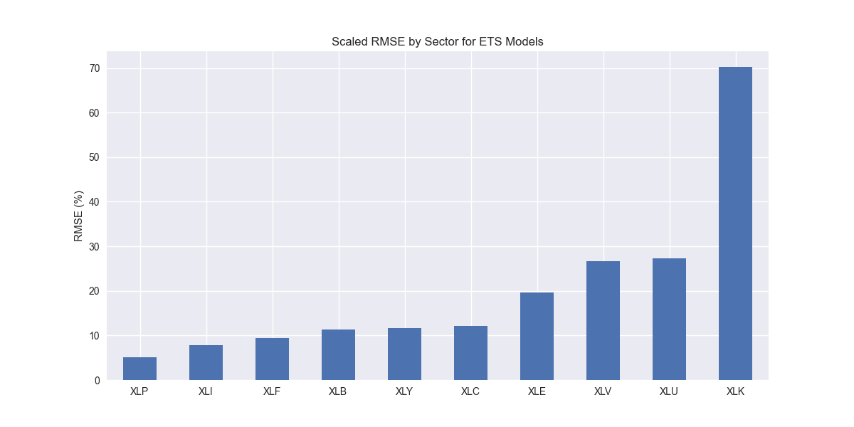
XLK, the technology sector, continues to suffer the highest error rate among all the others. This is mainly due to Nvidia (NVDA), which we've explained before here. Still it’s lower than other models and the next highest error rate is also lower. Let's move on to the comparison with benchmarks.

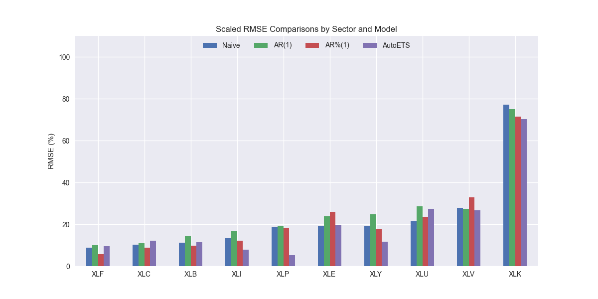
It appears AutoETS produces models with a generally lower error than the naive model on XLI, XLK, XLV, XLP, and XLY, the industrials, technology, healthcare, staples, and discretionary ETFs. For the remainder, it's worse. But the differences are modest. Let's confirm the aggregate performance below.

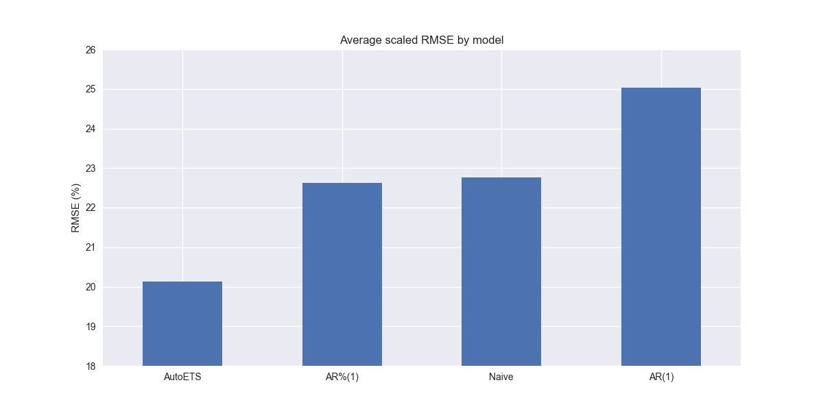
Wow! AutoETS really knocks the cover off the ball. Of course, our scaling makes the performance appear more dramatic than it really is. Nonetheless, aggregate performance is 2% points better than the naive and autoregressive growth (AR%(1)) benchmarks. We have a new winner.

While this is indeed encouraging, we should note that we're now moving into the realm where explainability starts to slip. Sure we can drill down into each model to call the individual parameters. But, instead of one set we now have 50 and who knows how many share the same set of multiplicative, additive, or none classifications? That is something we'll address in our next post. Or should it be our next, next post? We have a lot in the pipeline. If you have a preference, let us know in the comments below or send an email to content at optionstocksmachines dot com. Stay tuned!

Code below

# Load packages
import numpy as np
import pandas as pd
from datetime import datetime, timedelta
import statsmodels.api as sm
import matplotlib.pyplot as plt
from matplotlib.ticker import FuncFormatter
import matplotlib as mpl
import pickle
from sktime.forecasting.ets import AutoETS

# Assign chart style
plt.style.use('seaborn-v0_8')
plt.rcParams["figure.figsize"] = (12,6)

# Handy functions
# Functions to load and save files
def save_dict_to_file(data, filename):
    with open(filename, 'wb') as f:
        pickle.dump(data, f)

def load_dict_from_file(filename):
    with open(filename, 'rb') as f:
        return pickle.load(f)

# Create functions for indexing
def create_index(series):
    if series.iloc[0] > 0:
        return series/series.iloc[0] * 100
    else:
        return (series - series.iloc[0])/-series.iloc[0] * 100

# Function for scaled RMSE
def get_rmse_scaled(series):
    return np.sqrt(np.mean((series['actual']-series['predicted'])**2))/np.mean(series['actual'])

# Function to flatten
def flatten_df(dataf: pd.DataFrame, group_name:str, cols:list) -> pd.DataFrame:
    df_grouped = dataf.groupby(group_name)[cols].agg(list)

    for col in cols:
        df_grouped[col] = df_grouped[col].apply(lambda x: np.concatenate(x))
    
    df_long = df_grouped.apply(pd.Series.explode).reset_index()

    return df_long

# Symbols used
etf_symbols = ['XLF', 'XLI', 'XLE', 'XLK', 'XLV', 'XLY', 'XLP', 'XLB', 'XLU', 'XLC']

ticker_list = ["SHW", "LIN", "ECL", "FCX", "VMC",
               "XOM", "CVX", "COP", "WMB", "SLB",
               "JPM", "V", "MA", "BAC", "GS",
               "CAT", "RTX", "DE", "UNP", "BA",
               "AAPL", "MSFT", "NVDA", "ORCL", "CRM",
               "COST", "WMT", "PG", "KO", "PEP",
               "NEE", "D", "DUK", "VST", "SRE",
               "LLY", "UNH", "JNJ", "PFE", "MRK",
               "AMZN", "SBUX", "HD", "BKNG", "MCD",
               "META", "GOOG", "NFLX", "T", "DIS"
]

xlb = ["SHW", "LIN", "ECL", "FCX", "VMC"]
xle = ["XOM", "CVX", "COP", "WMB", "SLB"]
xlf = ["JPM", "V", "MA", "BAC", "GS"]
xli = ["CAT", "RTX", "DE", "UNP", "BA"]
xlk = ["AAPL", "MSFT", "NVDA", "ORCL", "CRM"]
xlp = ["COST", "WMT", "PG", "KO", "PEP"]
xlu = ["NEE", "D", "DUK", "VST", "SRE"]
xlv = ["LLY", "UNH", "JNJ", "PFE", "MRK"]
xly = ["AMZN", "SBUX", "HD", "BKNG", "MCD"]
xlc = ["META", "GOOG", "NFLX", "T", "DIS"]

sectors = [xlf,  xli,  xle,  xlk, xlv,  xly, xlp, xlb, xlu, xlc]

# Sector dictionary
sector_dict = {symbol.lower(): tickers for symbol, tickers in zip(etf_symbols, sectors)}
sector_map = {ticker.lower(): symbol for symbol, tickers in zip(etf_symbols, sectors) for ticker in tickers}

# Load data from disk
# See Code Walk-Throughs for how we built the data set
df_sector_dict = load_dict_from_file("path/to/data/simfin_df_rev_dict.pkl")

# Clean dataframes
df_rev_index_dict = {}
for key in sector_dict:
    temp_df = df_sector_dict[key].copy()
    col_1 = temp_df.columns[0]
    temp_df = temp_df[[col_1] + [x for x in temp_df.columns if 'revenue' in x]]
    temp_df.columns = ['date'] + [x.replace('revenue_', '').lower() for x in temp_df.columns[1:]]
    temp_idx = temp_df.copy()
    temp_idx[[x for x in temp_idx if 'date' not in x]] = temp_idx[[x for x in temp_idx if 'date' not in x]].apply(create_index)
    df_rev_index_dict[key] = temp_idx

# Create train/test dataframes
df_rev_train_dict = {}
df_rev_chg_train_dict = {}
df_rev_test_dict = {}
for key in df_rev_index_dict:
    # Create ticker list
    tickers = [x.lower() for x in sector_dict[key]]
    
    # Create dataframe fo all
    df_out = df_rev_index_dict[key]

    # Base train df
    df_train = df_out.loc[df_out['date'] < "2023-01-01"].copy()
    df_rev_train_dict[key] = df_train
    
    # Chang train df
    df_train_chg = df_train.copy()
    df_train_chg[tickers] = df_train_chg[tickers].apply(lambda x: np.log(x).diff())
    df_train_chg = df_train_chg.dropna()
    df_rev_chg_train_dict[key] = df_train_chg

    # Test df
    df_rev_test_dict[key] = df_out.loc[df_out['date'] >= "2023-01-01"]

# Create trend models
auto_ets_models = {}
for key in df_rev_chg_train_dict:
    tickers = [x.lower() for x in sector_dict[key]]
    df_train = df_rev_train_dict[key]
    auto_ets_models[key] = {}
    for ticker in tickers:
        try: 
            model = AutoETS(
                auto=True,
                n_jobs=-1,
                sp=4          
            ).fit(df_train[ticker])
 
        except ValueError as e:
            print(f"{ticker} fails due to {e}")

        auto_ets_models[key][ticker] = model

auto_ets_err_df = pd.DataFrame(columns = ['sector', 'ticker', 'actual', 'predicted'])
count = 0

fh = np.arange(1,5)
for key in auto_ets_models:
    for ticker in auto_ets_models[key]:
        
        # Forecast the next 4 quarters
        y_pred = auto_ets_models[key][ticker].predict(fh)
        y_act = df_rev_test_dict[key][ticker].values

        auto_ets_err_df.loc[count] = [key.upper(), ticker, y_act, y_pred]
        count += 1

for ticker in auto_ets_err_df['ticker'].to_list():
    actual = auto_ets_err_df.loc[auto_ets_err_df['ticker']==ticker, 'actual'].values[0]
    predicted = auto_ets_err_df.loc[auto_ets_err_df['ticker']==ticker, 'predicted'].values[0]
    rmse = np.sqrt(np.mean((actual - predicted)**2))
    rmse_scaled = rmse/actual.mean()
    auto_ets_err_df.loc[auto_ets_err_df['ticker']==ticker, 'rmse'] = rmse
    auto_ets_err_df.loc[auto_ets_err_df['ticker']==ticker, 'rmse_scaled'] = rmse_scaled
  
# Clean and flatten ar_err_df
auto_ets_df_long = flatten_df(auto_ets_err_df, 'sector', ['actual', 'predicted'])

# Graph scaled RMSE by sector
(auto_ets_df_long.groupby('sector')[['actual', 'predicted']].apply(get_rmse_scaled).sort_values(ascending=True)*100).plot(kind='bar', rot=0)
plt.xlabel('')
plt.ylabel('RMSE (%)')
plt.title('Scaled RMSE by Sector for ETS Models')
# plt.savefig("hello_world/images/day_20_autoets_rmse.png")
plt.show()

comp_df = pd.read_pickle("hello_world/data/comp_new_df.pkl")
auto_ets = auto_ets_df_long.groupby('sector')[['actual', 'predicted']].apply(get_rmse_scaled).reset_index().rename(columns={0:'auto_ets'})
comp_df = comp_df.merge(auto_ets, how="left", on='sector')
comp_df.iloc[:, 1:].mean()*100

# Plot RMSE by sector and model  
(comp_df.set_index('sector')[['naive', 'lr', 'chg','auto_ets']].sort_values('naive')*100).plot(kind='bar', rot=0)
plt.xlabel('')
plt.ylabel('RMSE (%)')
plt.ylim(0, 110)
plt.legend(['Naive', 'AR(1)', 'AR%(1)', 'AutoETS'], loc='upper center', ncol=4)
plt.title('Scaled RMSE Comparisons by Sector and Model')
plt.show()

# Plot Average performance
x_lab_dict = {'naive': 'Naive', 'lr': 'AR(1)', 'chg': 'AR%(1)', 'auto_ets':'AutoETS'}
x_labs = comp_df.iloc[:, 1:].mean().sort_values().index.to_list()

(comp_df.iloc[:, 1:].mean().sort_values()*100).plot(kind='bar', rot=0)
plt.xticks(np.arange(4), [x_lab_dict[x] for x in x_labs])
plt.ylabel('RMSE (%)')
plt.ylim(18,26)
plt.title('Average scaled RMSE by model')
plt.show()

# Comparisons
comp_df.loc[comp_df['auto_ets']<comp_df['naive'], 'sector']
comp_df.loc[comp_df['auto_ets']>comp_df['naive'], 'sector']